
Chapter Relevance
Lab Relevance: ★★★ (Crucial for importing and accessing raster data in labs)
Project Relevance: ★★★ (Essential if your project relies on raster environmental grids)
Foundation: ★★★ (Core concept establishing the link between arrays and geographic space)
Time to Read: 15 minutes
In a nutshell: Learn how to use the Rasterio library to safely open GeoTIFF files, extract their numerical data into NumPy arrays, and access their critical spatial metadata.
Skip this if: You are fully comfortable opening rasters using the with rasterio.open() context manager, extracting bands with .read(), and retrieving metadata like .crs and .transform.
Data Preparation
To follow along with this chapter, place the following datasets in a data folder next to your notebook:
1. What is Rasterio?
You have seen how NumPy powers the numerical calculations required for processing continuous grids. However, NumPy alone does not know how to open a GeoTIFF file, nor does it understand geographic coordinate reference systems.
To work with real spatial data, we need a translator. rasterio is a core Python library for reading and writing geospatial raster data. Built on top of the robust C++ geospatial library GDAL, Rasterio acts as the practical bridge between the physical raster files saved on your hard drive and the fast NumPy arrays you use for analysis in your computer’s memory.
2. Opening a Raster Safely
To access a raster file, you must open a connection to it. Because spatial datasets can be massive, it is critical to manage your computer’s memory responsibly.
You should open raster files using a Python with statement:
import rasterio

filepath = "data/Copernicus_DEM_NZ_subset.tif"

# Open the raster connection safely
with rasterio.open(filepath) as src:
    print(src.name)
    print(src.mode)
data/Copernicus_DEM_NZ_subset.tif
r
Using the with statement is a strict best practice. It creates a temporary context for the src object (the “source” dataset). The moment your code finishes executing the indented block, Rasterio automatically closes the file and releases the memory, even if an error occurs during processing.
Notice the output of src.mode. The 'r' stands for read-only. This is the default setting when opening a file, and it acts as a built-in safety feature. It guarantees that you can extract the data into NumPy without accidentally modifying or corrupting the original GeoTIFF on your hard drive. Later in the course, when you are ready to save your modified arrays back to disk, you will explicitly change this mode to 'w' (write).
3. Reading Bands into Arrays
Before extracting data, it helps to understand how raster files are physically structured. Many raster datasets consist of multiple layers called bands. For example, a satellite image often contains separate bands for Red, Green, Blue, and Near Infrared light.
Opening the dataset connection with rasterio.open() does not automatically load these millions of pixel values into your computer’s memory. You must explicitly extract the data you need using the .read() method.
Following standard geospatial conventions, Rasterio indexes bands starting at 1 (not 0).
with rasterio.open(filepath) as src:
    # Read the first band into memory
    elevation = src.read(1)

# The connection is now closed, but the data is safely stored
print(f"Type: {type(elevation)}")
print(f"Dimensions: {elevation.ndim}")
print(f"Shape: {elevation.shape}")
print(f"Data type: {elevation.dtype}")
Type: <class 'numpy.ndarray'>
Dimensions: 2
Shape: (2038, 2170)
Data type: float32
Notice the critical transition here: src was a Rasterio dataset object, but elevation is purely a standard numpy.ndarray. You have successfully crossed the bridge into the familiar territory of NumPy matrix math.
This physical structure connects directly to your array dimensions:
Reading a single specific band using
.read(1)creates a two dimensional NumPy array of rows and columns.If you read the entire multiband dataset at once using
.read(), Rasterio creates a three dimensional NumPy array stacked by bands, rows, and columns.
Concept Check: Properties of the Array vs. Dataset
Scenario: You successfully open a GeoTIFF file and read the first band into a NumPy array using data = src.read(1). To verify the geographic projection of your new array, you type print(data.crs). What happens?
A) Python prints the EPSG code of the map projection (e.g., “EPSG:4326”).
B) Python throws an AttributeError.
C) Python returns the mathematical transform matrix.
Check your understanding
Answer: B
Python will throw an AttributeError because data is a pure NumPy array, which only understands rows, columns, and numbers. It has no .crs attribute. The spatial projection, coordinate system, and all other geographical properties are securely stored within the original Rasterio dataset object (src), not the extracted array!
4. Quick Visual Feedback
Once your data is loaded into memory, you should verify it visually before starting any complex analysis. Rasterio provides a dedicated plotting module that renders spatial arrays correctly.
from rasterio.plot import show

with rasterio.open(filepath) as src:
    # Display the raster directly from the source object
    show(src, title="New Zealand Elevation DEM", cmap="terrain")
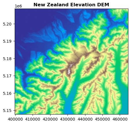
This show() function allows you to quickly spot missing data values or confirm you loaded the correct geographic region.
5. The Missing Geography: Raster Metadata
We have reached a critical conceptual pivot point.
If you only look at the extracted elevation array, the top-left pixel is simply located at row 0, column 0.
How does the computer know where this specific array actually sits on the Earth? How does it know whether the grid cells represent 10-meter squares in New Zealand or 30-meter squares in Switzerland?
The NumPy array itself does not know. To answer these questions, we need metadata.
The Geo in the Grid
The spatial meaning of the array is securely stored inside the Rasterio dataset object (src), not inside the extracted NumPy array.
You can access all the critical spatial information at once using the .meta or .profile attributes. This returns a dictionary containing everything Rasterio knows about the file’s spatial footprint.
with rasterio.open(filepath) as src:
    metadata = src.meta

print(metadata)
{'driver': 'GTiff', 'dtype': 'float32', 'nodata': None, 'width': 2170, 'height': 2038, 'count': 1, 'crs': CRS.from_wkt('PROJCS["WGS 84 / UTM zone 59S",GEOGCS["WGS 84",DATUM["WGS_1984",SPHEROID["WGS 84",6378137,298.257223563,AUTHORITY["EPSG","7030"]],AUTHORITY["EPSG","6326"]],PRIMEM["Greenwich",0,AUTHORITY["EPSG","8901"]],UNIT["degree",0.0174532925199433,AUTHORITY["EPSG","9122"]],AUTHORITY["EPSG","4326"]],PROJECTION["Transverse_Mercator"],PARAMETER["latitude_of_origin",0],PARAMETER["central_meridian",171],PARAMETER["scale_factor",0.9996],PARAMETER["false_easting",500000],PARAMETER["false_northing",10000000],UNIT["metre",1,AUTHORITY["EPSG","9001"]],AXIS["Easting",EAST],AXIS["Northing",NORTH],AUTHORITY["EPSG","32759"]]'), 'transform': Affine(30.0, 0.0, 399660.0,
       0.0, -30.0, 5208780.0)}
This metadata dictionary is vital. When you finish crunching numbers in NumPy and want to save your results as a new GeoTIFF, you must pass this metadata back to Rasterio so the new file retains its correct geographic positioning.
Coordinate Reference System and Bounds
While the .meta dictionary gives you everything at once, you can also inspect specific spatial attributes individually.
Just like GeoPandas vector layers, every spatial raster has a Coordinate Reference System (CRS). You can also inspect the .bounds, which define the exact bounding box and spatial extent the raster covers.
with rasterio.open(filepath) as src:
    print(f"CRS: {src.crs}")
    print(f"Bounds: {src.bounds}")
CRS: EPSG:32759
Bounds: BoundingBox(left=399660.0, bottom=5147640.0, right=464760.0, top=5208780.0)
The Affine Transform
The most important piece of spatial metadata is the .transform.
The transform is the mathematical engine that links simple pixel positions (like row 5, column 10) to real-world coordinates (like Easting and Northing).
Keep the concept practical: the NumPy array provides the row and column positions. The transform tells the computer exactly where the top-left corner of the image is located in space, and exactly how large each pixel is.
To understand how this mathematical mapping works without writing complex formulas, explore the interactive transform visualizer below.
Interactive Explorer: Affine Transform Visualizer.
Click different pixels within the Raster Matrix to observe how the Affine Transform acts as a mathematical bridge. It instantly converts the row and column indices of a "dumb" array into precise real-world geographic coordinates using the origin point and pixel size. For improved visibility of the explorer, follow this link.
6. Exercise: Open, Read, and Inspect
Now it is time to combine everything you have learned into a single, complete workflow.
You are given a multispectral satellite image subset: data/LC09_L1TP_075090_20230224_20230308_02_T1_subset.tif.
Tasks:
Open the raster safely using a
withstatement.Read the fourth band (Near Infrared) into a NumPy array named
band4.Print the
.shapeand.dtypeof the NumPy array.Print the
.crs,.bounds, and.transformof the Rasterio dataset object.Use
show()to plot the extracted band.
# Write your code here
Sample Solution
import rasterio
from rasterio.plot import show

filepath = "data/LC09_L1TP_075090_20230224_20230308_02_T1_subset.tif"

# 1. Open the raster safely
with rasterio.open(filepath) as src:

    # 2. Read the fourth band (NIR)
    band4 = src.read(4)

    # 3. Print array properties
    print("--- NumPy Array Properties ---")
    print(f"Shape: {band4.shape}")
    print(f"Data type: {band4.dtype}\n")

    # 4. Print spatial metadata
    print("--- Spatial Metadata ---")
    print(f"CRS: {src.crs}")
    print(f"Bounds: {src.bounds}")
    print(f"Transform:\n{src.transform}\n")

# 5. Plot the dataset (outside the block is fine since the array is in memory)
show(band4, title="Landsat 9 - Band 4 (NIR)", cmap="gray")
Output:
--- NumPy Array Properties ---
Shape: (2038, 2170)
Data type: float32

--- Spatial Metadata ---
CRS: EPSG:32759
Bounds: BoundingBox(left=399660.0, bottom=5147640.0, right=464760.0, top=5208780.0)
Transform:
| 30.00, 0.00, 399660.00|
| 0.00,-30.00, 5208780.00|
| 0.00, 0.00, 1.00|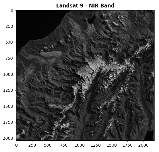
Output: Visualizing the Near Infrared band. Because we loaded the data into a standard NumPy array, we can easily apply Matplotlib colormaps like gray to enhance contrast.
7. Summary: From File to Spatial Array
Understanding the division of labor between Rasterio and NumPy is the key to spatial programming in Python.
Rasterio handles the heavy lifting of opening geospatial files from your hard drive.
The
.read()method translates physical raster bands into clean NumPy arrays.The NumPy array holds the actual environmental values (the numbers you crunch).
The Rasterio dataset object securely holds the metadata (the geography).
You need both components to perform meaningful spatial analysis. In the next chapters, you will see how to manipulate these numerical arrays and save your modified landscapes back to disk.