
Chapter Relevance
Lab Relevance: ★★★ (Fundamental for all raster-based labs)
Project Relevance: ★★☆ (Crucial if your project incorporates environmental or satellite data)
Foundation: ★★★ (The absolute foundation for Python numerical computing)
Time to Read: 15 minutes
In a nutshell: Learn the core mechanics of NumPy arrays, including creation, slicing, broadcasting, and aggregation, to understand the mathematical engine behind raster data.
Skip this if: You are highly proficient with NumPy arrays, slicing, boolean masking, and vectorized array mathematics.
1. From Lists to Arrays
To work with raster data in Python, you first need to understand the data structure that powers it. NumPy, short for Numerical Python, is the core library for numerical computing in Python. Its central object is the array, a fast and efficient structure for storing and manipulating large grids of numbers.
This matters because a raster band is, at its core, just a two dimensional array of values. Each cell stores a measurement for one location, such as elevation, temperature, or reflectance. If you want to work with raster data effectively, you need to be comfortable working with arrays.
You could store pixel values in ordinary Python lists, but lists are not designed for large scale numerical work. NumPy arrays are. They make calculations faster, cleaner, and easier to express.
The most important shift in thinking is this: operations on NumPy arrays are usually applied element by element. If you multiply an array by 2, NumPy multiplies every value in the grid by 2. This lets you transform entire surfaces at once without writing repetitive loops.
2. Creating Arrays and Grids
By convention, NumPy is usually imported with the alias np.
import numpy as np
Understanding dimensions
A useful way to think about a NumPy array is as a structured grid of values.
A one dimensional array looks much like a list.
A two dimensional array looks like a table.
A three dimensional array can be imagined as a stack of tables.
NumPy generalizes this idea to any number of dimensions. That is why its core array class is called ndarray, short for N dimensional array.
Most NumPy arrays follow a few important rules:
all elements have the same data type
the overall size does not change after creation
the shape is regular, not jagged
These restrictions are helpful. They allow NumPy to store data efficiently and perform calculations much faster than standard Python lists.
Creating arrays
You can create a NumPy array directly from a Python list using np.array().
arr_1d = np.array([1, 2, 3, 4])
arr_2d = np.array([[1, 2], [3, 4]])

print("1D array:")
print(arr_1d)

print("\n2D array:")
print(arr_2d)
1D array:
[1 2 3 4]

2D array:
[[1 2]
 [3 4]]
When working with raster like data, you often want to begin with a blank grid. NumPy provides simple ways to generate these starting structures:
np.zeros()creates an array filled with zerosnp.ones()creates an array filled with onesnp.arange()creates a regular numeric sequence
zeros = np.zeros((3, 3))
ones = np.ones((2, 4))
sequence = np.arange(0, 10, 2)

print("Zeros:\n", zeros)
print("\nOnes:\n", ones)
print("\nSequence:\n", sequence)
Zeros:
 [[0. 0. 0.]
 [0. 0. 0.]
 [0. 0. 0.]]

Ones:
 [[1. 1. 1. 1.]
 [1. 1. 1. 1.]]

Sequence:
 [0 2 4 6 8]
arange() vs. linspace()
Both np.arange() and np.linspace() create sequences, but they work a little differently.
Use
np.arange()when you want to control the step sizeUse
np.linspace()when you want to control the number of values
Here is a simple example with linspace():
values = np.linspace(0, 10, num=5)
print(values)
[ 0. 2.5 5. 7.5 10. ]
This creates five evenly spaced values between 0 and 10, including both endpoints.
Reshaping arrays
Once you have created a one dimensional sequence, you can reorganize it into a two dimensional grid using reshape().
This is especially useful when flat data need to be turned into a matrix.
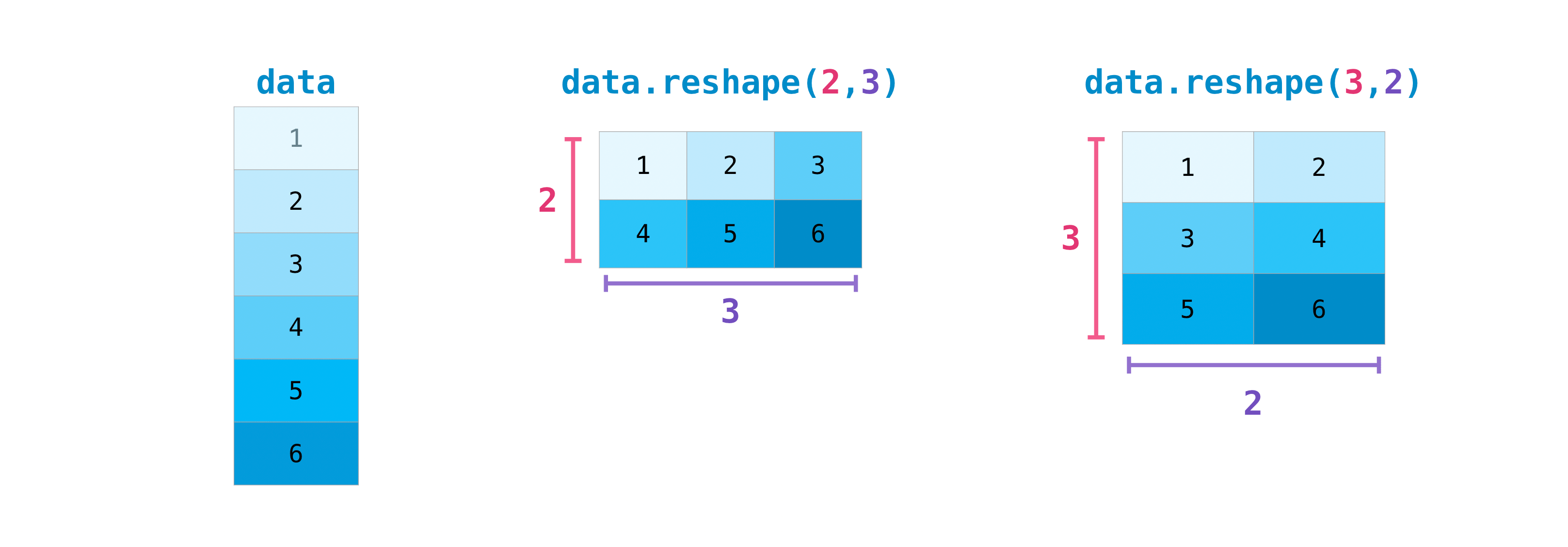
*Visualizing array restructuring: A one dimensional sequence of 6 elements can be instantly reshaped into a grid of 2 rows and 3 columns, or 3 rows and 2 columns. Source: Numpy*
# Create a 1D sequence from 1 to 6
data = np.arange(1, 7)

# Reshape the data sequence into a 2x3 grid
grid_2x3 = data.reshape((2, 3))
print("2x3 grid:\n", grid_2x3)

# Reshape the same data sequence into a 3x2 grid
grid_3x2 = data.reshape((3, 2))
print("\n3x2 grid:\n", grid_3x2)
2x3 grid:
 [[1 2 3]
 [4 5 6]]

3x2 grid:
 [[1 2]
 [3 4]
 [5 6]]
A result like this is already starting to look like a tiny raster band: a regular grid of values arranged by rows and columns. At this stage, however, it is still just a numerical array. The spatial meaning comes later, when coordinates, resolution, and other raster metadata are added.
3. Array Properties
Whenever you create or load a new array, it is good practice to inspect its basic structure first. This helps you confirm exactly what kind of object you are working with and how the data is organized.
You can use the built-in Python type() function to confirm that the object is indeed a NumPy array. After that, four key attributes will tell you everything you need to know about the array’s geometry:
.ndim: Tells you the number of dimensions the array has. For example, a flat sequence is 1D, while a spatial grid is 2D..shape: Returns a tuple specifying the number of elements along each dimension. For a 2D array, this represents the number of rows and columns (for example,(3, 4))..size: Tells you the fixed, total number of individual elements inside the entire array..dtype: Because NumPy arrays are typically homogeneous (containing elements of only one data type), this attribute tells you exactly what kind of data is stored inside, such as integers or floats.
This quick “first check” is one of the most useful debugging habits you can build before you start performing map algebra on large raster datasets.
print(f"Type: {type(grid_3x2)}")
print(f"Dimensions: {grid_3x2.ndim}")
print(f"Shape: {grid_3x2.shape}")
print(f"Size: {grid_3x2.size}")
print(f"Data type: {grid_3x2.dtype}")
Type: <class 'numpy.ndarray'>
Dimensions: 2
Shape: (3, 2)
Size: 6
Data type: int64
4. Indexing, Slicing, and Updating
One of NumPy’s greatest strengths is that it makes it easy to access, extract, and modify selected parts of an array. This is essential for raster work, where you often want to inspect a single cell, extract an analysis window, or update a group of pixels.
NumPy arrays are zero-indexed, so the first row and first column both start at index 0.
Indexing in one dimension
Before working with grids, it helps to recall how indexing works in a simple one dimensional array.
data = np.array([1, 2, 3, 4, 5, 6])

print(data[0])  # first value
print(data[1])  # second value
print(data[0:2])  # first two values
print(data[3:])  # everything from index 3 onward
print(data[-2:])  # last two values
1
2
[1 2]
[4 5 6]
[5 6]
![Diagram showing how a 1D array can be sliced using indices like data[0:2], data[1:], and data[-2:].](/sds210-jb/build/03_np_indexing-19816f6d6be0a340ae6f1ce839300a14.png)
*Visualizing array slicing: You can use start and end indices to extract specific sections of an array. Source: Numpy*
An important rule in Python slicing is that the stop value is excluded. So data[0:2] includes indices 0 and 1, but never 2.
Accessing single values in two dimensions
In a two dimensional array, you specify both the row and column position inside one pair of square brackets.
grid = np.array([[1, 2, 3], [4, 5, 6], [7, 8, 9]])

# Access the element in the first row and second column
value = grid[0, 1]
print(value)
2
Slicing rows, columns, and windows
Slicing lets you extract subsets of an array using the : symbol. In two dimensions, you can slice rows and columns at the very same time.
# Slice the first two rows and all columns
top_rows = grid[:2, :]

# Slice from row 1 onward, and the first two columns
bottom_left_window = grid[1:, :2]

# Slice a 2x2 window from the upper left
window = grid[:2, :2]

# Slice a rectangular inner window
inner_window = grid[1:3, 1:3]

print("Top rows:\n", top_rows)
print("\nBottom left window:\n", bottom_left_window)
print("\n2x2 window:\n", window)
print("\nRectangular inner window:\n", inner_window)
Top rows:
 [[1 2 3]
 [4 5 6]]

Bottom left window:
 [[4 5]
 [7 8]]

2x2 window:
 [[1 2]
 [4 5]]

Rectangular inner window:
 [[5 6]
 [8 9]]
This is the foundational pattern for extracting analysis windows or cropping regions of interest from large raster files.
Concept Check: The Missing Pixel
Scenario: You have a 1D array of 5 pixel values: data = np.array([10, 20, 30, 40, 50]). You want to extract the second and third pixels (the values 20 and 30). Which slice must you use?
A) data[1:2]
B) data[2:3]
C) data[1:3]
Check your understanding
Answer: C
In Python, arrays are zero-indexed, meaning the second pixel is at index 1. Furthermore, slicing is exclusive of the stop value. Therefore, data[1:3] extracts indices 1 and 2, safely stopping before it hits index 3.
Updating values
You can use indexing and slicing not only to read values, but also to instantly change them.
# Set a specific cell to 10
grid[2, 2] = 10

# Update a 2x2 window to 5
grid[0:2, 0:2] = 5

print(grid)
[[ 5  5  3]
 [ 5  5  6]
 [ 7  8 10]]
Boolean indexing
NumPy also allows you to select values based on specific mathematical conditions. This is called boolean indexing.
a = np.array([[1, 2, 3, 4], [5, 6, 7, 8], [9, 10, 11, 12]])

print(a[a < 5])
print(a[a >= 5])
[1 2 3 4]
[ 5  6  7  8  9 10 11 12]
A condition such as a < 5 actually creates a temporary boolean array of the exact same shape, filled entirely with True and False values. NumPy then applies that mask over your original array to return only the matching values.
This technique is very useful for thresholding or isolating pixels.
You can also combine multiple conditions using & (and) or | (or):
selected = a[(a > 2) & (a < 11)]
print(selected)
[ 3 4 5 6 7 8 9 10]
This kind of targeted updating is useful when simulating terrain, applying masks, or changing selected raster cells.
Interactive Explorer: Array Slicing and Masking.
Toggle between modes to explore how array slicing and boolean masking extract specific data from a 2D grid. Adjust the row and column boundaries or the boolean threshold, and watch the visual selection instantly update alongside the corresponding NumPy syntax. For improved visibility of the explorer, follow this link.
5. Array Math & Summaries
NumPy is powerful because it lets you apply mathematical operations to entire arrays at once.
Scalar and element-wise math
If you combine an array with a single number (a scalar), NumPy automatically applies that operation to every cell in the array. This concept is called broadcasting.
grid = np.array([[1, 2, 3], [4, 5, 6], [7, 8, 9]])

# Scalar math (Broadcasting): multiply all pixels by 2
doubled_grid = grid * 2

# Scalar math: add 10 to all pixels
offset_grid = grid + 10

print("Doubled Grid:\n", doubled_grid)
print("\nOffset Grid:\n", offset_grid)
Doubled Grid:
 [[ 2  4  6]
 [ 8 10 12]
 [14 16 18]]

Offset Grid:
 [[11 12 13]
 [14 15 16]
 [17 18 19]]
You can also perform element-wise math between two arrays, provided they have compatible dimensions (e.g., the same shape). This is useful for operations like calculating the difference between two raster layers (e.g., finding elevation change over time).
# Element-wise addition
combined_grid = grid + offset_grid

print("Combined Grid:\n", combined_grid)
Combined Grid:
 [[12 14 16]
 [18 20 22]
 [24 26 28]]
Mathematical functions
NumPy includes a vast library of ready-made mathematical functions (often called universal functions or ufuncs) that work directly on arrays.
# Apply a logarithmic transformation (log(1 + x) handles zeros safely)
log_grid = np.log1p(grid)

# Or calculate the square root of every pixel
sqrt_grid = np.sqrt(grid)

# Or perform trigonometry (e.g., when calculating terrain slope/aspect)
sin_grid = np.sin(grid)
This is especially useful in spatial data science, where raster processing often involves transforming values before analysis or visualization.
Summary statistics (Aggregation)
Once you have a grid of values, you often want quick summaries. NumPy provides aggregation functions like min, max, sum, mean, and std (standard deviation).
By default, these functions evaluate the entire array.
print(f"Min elevation: {grid.min()}")
print(f"Max elevation: {grid.max()}")
print(f"Sum of elevation: {grid.sum()}")
print(f"Mean elevation: {grid.mean()}")
print(f"Median elevation: {np.median(grid)}")
print(f"Standard deviation: {np.std(grid).round(2)}")
Min elevation: 1
Max elevation: 9
Sum of elevation: 45
Mean elevation: 5.0
Median elevation: 5.0
Standard deviation: 2.58
Aggregating along an axis
You can also calculate statistics for specific dimensions by specifying an axis. For a 2D array:
axis=0aggregates down the columns (vertically).axis=1aggregates across the rows (horizontally).
# Find the maximum value in each column
max_per_col = grid.max(axis=0)

# Find the mean value of each row
mean_per_row = grid.mean(axis=1)

print("Max value per column:", max_per_col)
print("Mean value per row:", mean_per_row)
Max value per column: [7 8 9]
Mean value per row: [2. 5. 8.]
These kinds of targeted summaries are very common in raster analysis, for example, when creating zonal statistics or analyzing temporal data where one axis represents time.
Concept Check: The Loop Bottleneck
Scenario: You have a high-resolution satellite image with 10 million pixels representing temperature. You need to convert the temperature from Celsius to Fahrenheit. Why shouldn’t you use a standard Python for loop to iterate through every pixel?
A) for loops cannot access pixel values; you must use a spatial join.
B) Standard Python lists and loops are not optimized for massive matrices and will hit a severe performance wall.
C) The data is continuous, so you can only calculate the area, not the temperature.
Check your understanding
Answer: B Raster data relies on massive matrices. Standard Python loops iterate one by one, which takes far too long for millions of cells. NumPy solves this using ‘vectorization’, pushing operations down to optimized C code to compute the whole matrix almost instantly.
6. Exercise: A Tiny Elevation Raster
You are given a tiny elevation raster for a mountain valley. Your task is to build the grid, inspect its structure, and identify the higher ground that might remain dry during heavy rainfall.
Tasks:
Create a
6 x 6array filled with zeros.Raise the center
2 x 2cells to an elevation of5.Set one center cell to
9as the highest point.Check the array’s
.shape,.ndim, and.dtype.Slice out the center
4 x 4area.Raise the terrain by
2meters everywhere.Calculate the minimum, maximum, and mean elevation.
Create a Boolean mask for all cells with elevation greater than
4.Assign
np.nan(NaN) to one corner cell to represent missing data.
# Write your code here
Sample Solution
import numpy as np

# 1. Create a 6x6 array filled with zeros (default dtype is float64)
grid = np.zeros((6, 6))

# 2. Raise the center 2x2 cells to 5
grid[2:4, 2:4] = 5

# 3. Set one center cell to 9 as the highest point
grid[2, 2] = 9

# 4. Check shape, ndim, and dtype
print(f"Shape: {grid.shape}, Dimensions: {grid.ndim}, Data Type: {grid.dtype}")

# 5. Slice out the center 4x4 area
center_4x4 = grid[1:5, 1:5]
print("\nCenter 4x4:\n", center_4x4)

# 6. Raise the terrain by 2 meters everywhere (scalar math)
grid = grid + 2
print("\nRaised Terrain:\n", grid)

# 7. Calculate min, max, and mean
print(f"\nMin: {grid.min()}, Max: {grid.max()}, Mean: {np.round(grid.mean(), 2)}")

# 8. Create a Boolean mask for elevation > 4
mask = grid > 4
print("\nMask (Elevation > 4):\n", mask)

# 9. Assign np.nan to a corner cell to represent missing data
grid[0, 0] = np.nan
print("\nTerrain with missing data (NaN):\n", grid)
7. Summary
At this point, you have learned the core mechanics of NumPy arrays:
how to create them
how to inspect their structure
how to slice and update selected values
how to apply mathematical operations across entire grids
how to summarise and filter them
This is the numerical foundation of raster processing in Python. A basic NumPy array can already behave like a tiny raster band: it is a regular grid of values that can be manipulated and analysed as a surface.
What it still lacks is the spatial context. At the moment, your array knows nothing about where it is in the world, how large each cell is, or which coordinate reference system it belongs to.
That is the next step. You are not leaving arrays behind. You are simply about to add spatial metadata and geographic file handling on top of the same array mechanics you now understand.