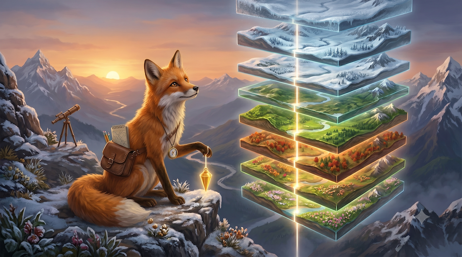
In the previous lesson, you learned how to process the environment as a continuous mathematical surface using Rasterio and NumPy. You transitioned from isolated vector shapes to millions of individual pixels, allowing you to quantify landscape features like vegetation density and spectral change.
That was an essential step for analyzing spatial surfaces, but it raises some new challenge:
What happens when your environment is not static?
Earth observation is fundamentally about change. You rarely want to look at just one satellite image; you want to look at tens, hundreds or even thousands of them stacked over months, years or decades to understand how a landscape is evolving.
This lesson introduces the final core paradigm of spatial data science: The Data Cube. Instead of analyzing single 2D grids, you will learn to navigate multidimensional spaces across space, time, and variables using the xarray library.
1. Meet multidimensional cubes
Programming time series analysis requires another major shift in your mental model.
If you stack 100 daily satellite images on top of each other, raw NumPy becomes incredibly difficult to manage. You would have to mentally track arbitrary numerical indices—trying to remember if “axis 0” is time or latitude, and calculating that “index 54” corresponds to June 4th. This leads to code that is unreadable and prone to silent errors.
Enter xarray. Xarray brings the intuitive labeling power of Pandas directly to the multidimensional matrix operations of NumPy.
Instead of guessing raw indices, you will interrogate the data cube using real-world labels. You will transition from writing matrix[54, 45, 120] to writing .sel(time="2023-06-04", lat=47.3). Your spatial and temporal metadata will be perfectly preserved, allowing you to slice, aggregate, and mathematically model decades of data with human-readable logic.
2. Why this matters for SDS
In spatial data science, time is the dimension that turns observation into insight.
Without time series analysis, you can map where a forest is. With it, you can measure exactly how fast it is expanding or degrading. Tracking dynamic processes, like accelerating ocean warming, shrinking Alpine snowpacks, or shifting seasonal cycles, requires you to handle time as a fluid, reducible dimension.
Mastering multidimensional data cubes allows you to answer complex climatological and environmental questions: How do we isolate a long-term global warming trend from the noisy cycle of summer and winter? How do we calculate the exact rate of snow decline at different mountain elevations?
By combining xarray with statistical modeling, you transition from simply drawing maps of the past to quantifying the rate of environmental change for the future.
3. Learning objectives
After this lesson, you will be able to:
Shift to the Data Cube model Understand the structural difference between
DataArrayandDatasetcontainers, and why label-based indexing is infinitely safer than pure NumPy indexing.Interrogate multidimensional space Extract precise 1D temporal signals from 3D arrays, apply complex boolean masks, and reduce regions into spatial summaries using the
.sel()and.where()methods.Execute aligned Raster Math Combine datasets (like DEMs and multispectral imagery) seamlessly, extracting ecological boundaries like treelines and snowlines by grouping variables together.
Visualize dynamic processes Generate faceted small-multiple maps, animate time dimensions into GIFs, and build interactive browser-native widgets using
hvplotandcartopy.Extract climatological signals Reorganize the time dimension using split-apply-combine workflows to calculate seasonal climatologies, extract historical anomalies, and apply rolling spatial weights.
Quantify long-term trends Apply pixel-wise linear and harmonic regressions (
.polyfitand.curvefit) across the globe simultaneously to extract definitive rates of environmental change.
4. Lesson structure
This lesson is structured to take you from the theoretical foundations of the cube to running robust climate regressions across the European Alps:
The Data Cube Model: Moving from flat 2D arrays to N-dimensional, label-aware containers.
Exploring the Cube: Reading, cleaning, formatting, and safely exporting massive datasets like NetCDF and Zarr.
Visualizing the Cube: Moving from quick static verification to multifaceted maps and interactive time-scrubbing dashboards.
Sampling the Cube: Interrogating data across precise temporal slices, geographic bounding boxes, and conditions.
Raster Math: Extracting environmental relationships by calculating indices and mapping variables against elevation.
Temporal Aggregation: Reorganizing time to isolate stable climate baselines and extract pure anomaly signals.
Long-Term Trends: Quantifying the mathematical rate of global change using vectorized linear and harmonic regressions.
Practical L10: Acting as a MeteoSwiss climatologist to calculate and map the decadal decline of snow cover across Alpine ski resorts.
5. Looking ahead
Lesson 10 is about temporal dynamics.
You will learn not only how to handle multi-layered rasters, but how to:
filter decades of noise to find the true underlying climate signal
seamlessly broadcast mathematical models across millions of pixels at once
extract highly specific insights from massive planetary datasets
If Lesson 9 was about analyzing every pixel, Lesson 10 is about watching every pixel evolve over time.
The multidimensional arrays and temporal modeling techniques you learn here are highly relevant for environmental monitoring. By fusing vector geometries, raw raster operations, and temporal data cubes, you now possess the toolkit necessary to track, quantify, and communicate the shifting realities of our planet.