
Chapter Relevance
Lab Relevance: ★★★ (Essential for exporting data to be used in GIS or other scripts)
Project Relevance: ★★★ (Required for saving outputs and managing data size in projects)
Foundation: ★★★ (Core spatial data management skills)
Time to Read: 15 minutes
In a nutshell: Master the mechanics of writing arrays back to disk with spatial metadata, handling massive files safely, and clipping data to areas of interest.
Skip this if: You are completely comfortable updating Rasterio profiles to write GeoTIFFs, using Window to read array subsets, and clipping arrays with vector geometries using rasterio.mask.
Data Preparation
To follow along with this chapter, place the following datasets in a data folder next to your notebook:
1. Writing Rasters
In the previous chapter, we used map algebra to calculate a binary snow mask from satellite imagery. However, that result currently exists only as a temporary NumPy array in your computer’s memory. To use this snow mask in geographic information systems (GIS) software or share it with colleagues, we must write it back to the hard drive as a spatial GeoTIFF.
Writing a standard image is simple, but a GeoTIFF requires strict spatial metadata. If we just save the NumPy array, it loses all geographic context and the output file will not know where it belongs on Earth. The golden rule of raster export is to always copy the .profile (the complete metadata dictionary) from your original input raster. This guarantees that your new output raster will perfectly align in space with the original dataset.
When you perform map algebra, you often change the fundamental structure of the data. For example, our input was a 7 band image of 16 bit integers, but our newly calculated snow mask is a single band of binary values (True or False). Exporting a simple binary mask as a 32 bit float is bad practice and wastes massive amounts of disk space. Instead, we should convert the boolean mask to an 8 bit unsigned integer (uint8) so it only stores zeros and ones.
Concept Check: The Bloated Export
Scenario: You have calculated a binary flood mask (values 0 and 1) from a 32-bit continuous elevation raster. You copy the original profile dictionary and instantly write the mask to disk using dst.write(mask, 1). Why might your output file be unnecessarily massive in size?
A) Binary masks inherently take up more disk space than continuous data because they cannot be compressed.
B) You did not convert the mask to a GeoDataFrame before exporting.
C) You forgot to update the profile’s dtype to uint8, meaning the file is allocating 32 bits of memory for every single 0 and 1.
Check your understanding
Answer: C
Because you copied the profile directly from a 32-bit elevation raster without updating it, Rasterio will write your simple 0 and 1 values as heavy 32-bit floats. By manually updating the profile with profile.update(dtype=rasterio.uint8), you ensure the file takes up the absolute minimum amount of hard drive space.
Before writing the file, we must update the copied profile dictionary to reflect these new data types. Additionally, to keep our project workspace organized, it is best practice to save all generated files into a dedicated folder rather than cluttering the main directory. We can use Python’s built-in os module to automatically create an outputs directory if it does not already exist.
Once the profile is updated and our output directory is ready, we open a new file connection using 'w' (write) mode, pass in the profile arguments, and use .write() to save the array to the hard drive.
import rasterio
import numpy as np
import os

input_path = "data/LC09_L1TP_075090_20230224_20230308_02_T1_subset.tif"

# Create a dedicated directory to organize our saved results
os.makedirs("outputs", exist_ok=True)
output_path = "outputs/snow_mask.tif"

with rasterio.open(input_path) as src:
    # Read bands and calculate the mask (from previous chapter)
    green = src.read(2).astype(float)
    nir = src.read(4).astype(float)
    swir2 = src.read(6).astype(float)

    with np.errstate(divide="ignore", invalid="ignore"):
        ndsi = (green - swir2) / (green + swir2)
        snow_mask = (ndsi * (nir > 0.2)) > 0.6

    # Convert boolean mask to an 8 bit integer (0 or 1) for efficient storage
    snow_mask = snow_mask.astype("uint8")

    # Copy the spatial profile
    profile = src.profile.copy()

# Update the profile to reflect the new data structure
profile.update(
    dtype=rasterio.uint8,
    count=1,  # We are only exporting 1 band
    compress="lzw",  # Apply lossless compression to save disk space
)

# Write to disk
with rasterio.open(output_path, "w", **profile) as dst:
    # Rasterio expects bands to be numbered starting at 1
    dst.write(snow_mask, 1)

print(f"Successfully saved {output_path}")
Successfully saved outputs/snow_mask.tif
2. Handling Large Datasets
Satellite imagery can be massive. A single full scene might be several gigabytes in size. Loading an entire file into memory with a simple .read() can easily overload your RAM and crash your computer. When working with large files, you must actively manage memory by processing the data efficiently.
Read one band: If you only need the Near Infrared band for your analysis, avoid loading the entire multispectral stack. Explicitly use
src.read(4)instead ofsrc.read().Use lower precision: Arrays consume memory based on their data type. A
float64array takes up twice as much RAM as afloat32array. Use.astype("float32")to downgrade precision if extreme decimal accuracy is not required.Read one window: You can load a small, specific bounding box of pixels into memory without touching the rest of the file using Rasterio’s
Windowclass.Process chunk by chunk: The most robust way to handle massive files is to loop through the raster in blocks. You open the file, read a small chunk into memory, process it, write that chunk directly to the new output file, and then move on to the next block.
from rasterio.windows import Window

with rasterio.open(input_path) as src:
    # Read an 800x800 pixel block starting from the top-left corner
    small_window = Window(col_off=0, row_off=0, width=800, height=800)
    chunk = src.read(1, window=small_window)

    print(f"Loaded chunk shape: {chunk.shape}")
Loaded chunk shape: (800, 800)
Once this subset is securely in memory, it behaves exactly like any other NumPy array. Before applying complex algorithms or map algebra to large datasets, it is highly recommended to visualize the extracted chunk to verify you grabbed the correct geographic area.
import matplotlib.pyplot as plt

plt.figure(figsize=(7, 7))
# We apply a contrast stretch using vmin and vmax for better visibility
plt.imshow(chunk, cmap="gray", vmin=0.05, vmax=0.2)
plt.title("Visualization of the 800x800 chunk", fontsize=15)
plt.colorbar(label="Pixel Value", fraction=0.046, pad=0.04)
plt.axis("off")
plt.show()
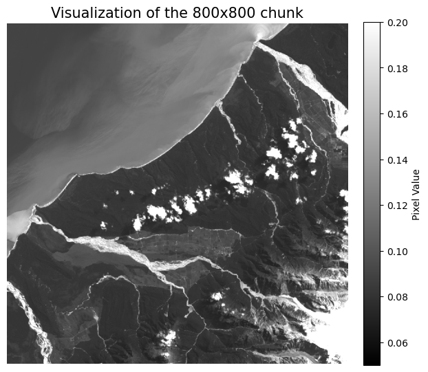
While manually defining a single window is perfect for targeted extraction, applying map algebra to an entire multi-gigabyte scene requires automation. You can bridge this gap and process a massive file sequentially using Rasterio’s built-in block_windows() iterator.
# Example: Looping through a massive dataset efficiently
with rasterio.open(input_path) as src:
    # Generate windows based on the internal tiling structure of Band 1
    for block_id, window in src.block_windows(1):
        # Read only the current chunk into memory
        chunk = src.read(1, window=window)

        # Process the chunk here (e.g., apply a math formula or index)
        # result = chunk * 2

        # In a full workflow, you would write 'result' to a destination
        # file using the exact same 'window' to maintain spatial alignment.
3. Clipping
Often, your study area is much smaller than the satellite scene you downloaded. Clipping restricts your analysis to a specific region, vastly reducing processing time and memory usage.
Slice the Array
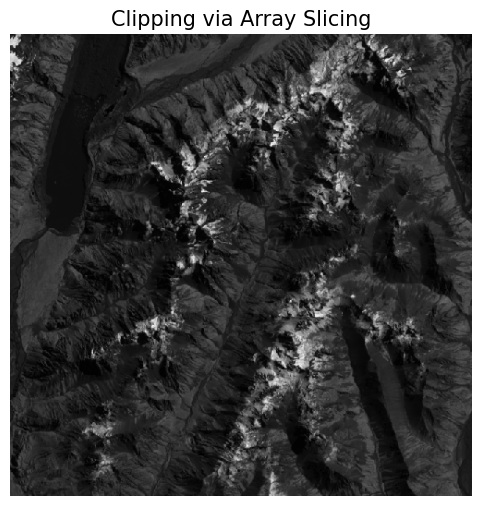
Because rasters are essentially NumPy arrays once read into memory, the fastest way to clip data is to simply slice the rows and columns using index numbers.
import rasterio
import matplotlib.pyplot as plt

with rasterio.open(input_path) as src:
    data = src.read(4)  # Read Band 4 (NIR)

# Slice the array: [rows, columns]
array_subset = data[1000:1500, 800:1300]

# Visualize the sliced subset
plt.figure(figsize=(6, 6))
plt.imshow(array_subset, cmap="gray")
plt.title("Clipping via Array Slicing", fontsize=15)
plt.axis("off")
plt.show()
Interactive Explorer: Raster Window Extractor.
Adjust the sliders to define a custom reading window within a standard Sentinel-2 image. Notice how extracting a specific spatial subset drastically reduces the required RAM, preventing memory crashes when dealing with massive satellite scenes. For improved visibility of the explorer, follow this link.
Use Geographic Bounds
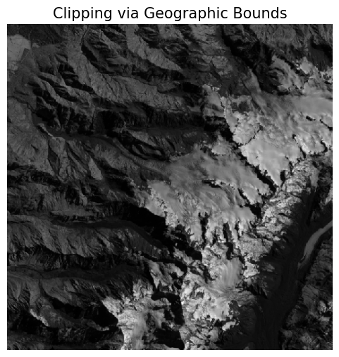
Slicing by pixel index is fast, but it is not geographically accurate. If you know the exact real-world coordinate bounding box of your study area, you can use Rasterio to safely convert those coordinates into a pixel window.
from rasterio.windows import from_bounds

with rasterio.open(input_path) as src:
    # Define your geographic bounding box (left, bottom, right, top)
    min_x, min_y, max_x, max_y = 420000, 5170000, 440000, 5190000

    # Create a window from geographic bounds using the raster's transform matrix
    geo_window = from_bounds(min_x, min_y, max_x, max_y, src.transform)

    # Read only the data within that calculated window
    geo_subset = src.read(4, window=geo_window)

plt.figure(figsize=(6, 6))
plt.imshow(geo_subset, cmap="gray")
plt.title("Clipping via Geographic Bounds", fontsize=15)
plt.axis("off")
plt.show()
Clip with a Shapefile
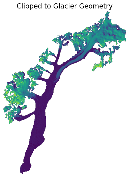
The most common and precise clipping method uses vector boundaries (polygons) to extract exact environmental features. In this example, we will clip our raster to the exact outline of the Haupapa/Tasman glacier in New Zealand (a glacier similar in size to the Aletsch glacier in Switzerland).
Rasterio provides a dedicated mask module to handle this complex geometry intersection.
import geopandas as gpd
import numpy as np
from rasterio.mask import mask

# 1. Load the vector boundary
glacier_gdf = gpd.read_file("data/GLIMS_haupapa_tasman.gpkg")

with rasterio.open(input_path) as src:
    # Ensure the vector data matches the raster CRS
    glacier_gdf = glacier_gdf.to_crs(src.crs)

    # Extract all shapes into a list directly from the geometry column
    shapes = glacier_gdf.geometry.tolist()

    # 2. Apply the mask. crop=True shrinks the array to the bounding box of the polygon.
    out_image, out_transform = mask(src, shapes, crop=True)

# Plot the clipped array
# Note: mask() returns all bands. Index 3 corresponds to Band 4 (NIR)
plt.figure(figsize=(7, 7))
nir_clipped = out_image[3]

# Replace 0 (the masked background) with NaN for a clean plot
nir_clean = np.where(nir_clipped == 0, np.nan, nir_clipped)

plt.imshow(nir_clean, cmap="viridis")
plt.title("Clipped to Glacier Geometry", fontsize=16)
plt.axis("off")
plt.show()
4. Reprojection
Different regions and datasets use different Coordinate Reference Systems (CRS) to minimize geographic distortion. For example, spatial data in Switzerland is commonly projected in local coordinates (LV95, EPSG:2056) or global zones (UTM32N, EPSG:32632).
Our current New Zealand dataset is in UTM Zone 59S (EPSG:32759). However, local environmental agencies primarily use the New Zealand Transverse Mercator (NZTM, EPSG:2193). To combine our snow mask with local government vector data, we must reproject our raster.
Reprojecting a raster is computationally intensive because the computer cannot simply stretch the image. It must recalculate the size, shape, and value of every individual pixel in a new mathematical grid—a process known as resampling. Rasterio handles this via its warp module, which acts as a Python wrapper around the powerful C++ library GDAL (Geospatial Data Abstraction Library). GDAL is the industry standard engine that powers almost all open-source geographic software (including QGIS).
Because we are warping the grid, we must first calculate the new dimensions and transformation matrix for the destination CRS before we can actually move the pixel values.
from rasterio.warp import calculate_default_transform, reproject, Resampling

input_raster = "outputs/snow_mask.tif"
dst_crs = "EPSG:2193"
output_raster = "outputs/snow_mask_nztm.tif"

with rasterio.open(input_raster) as src:
    # 1. Use GDAL engine to calculate the new dimensions and transform matrix
    # for the destination CRS based on the source boundaries
    transform, width, height = calculate_default_transform(
        src.crs, dst_crs, src.width, src.height, *src.bounds
    )

    # 2. Update the profile with the newly calculated spatial parameters
    profile = src.profile.copy()
    profile.update(
        {"crs": dst_crs, "transform": transform, "width": width, "height": height}
    )

    # 3. Write and reproject pixel by pixel
    with rasterio.open(output_raster, "w", **profile) as dst:
        reproject(
            source=rasterio.band(src, 1),
            destination=rasterio.band(dst, 1),
            src_transform=src.transform,
            src_crs=src.crs,
            dst_transform=transform,
            dst_crs=dst_crs,
            resampling=Resampling.nearest,
            # Nearest neighbor is critical here! It preserves our binary (0 or 1) values.
            # Using bilinear interpolation would create decimals (e.g., 0.45) at the edges.
        )

print("Reprojection complete.")
Reprojection complete.
5. Exercise: Extract and Export
Instead of reprojecting massive raster files, a standard spatial optimization is to reproject your lightweight vector boundaries to match the raster, clip the data, and then export the much smaller result.
Imagine a colleague needs a standalone GeoTIFF of the Near Infrared data (Band 4), restricted exactly to the boundaries of Lake Mapourika.
Tasks:
Open the Landsat subset (
LC09_L1TP_075090_20230224_20230308_02_T1_subset.tif) and load the Lake Mapourika vector (JRC_lake_mapourika.gpkg).Reproject the vector dataframe to match the raster’s CRS.
Use
rasterio.mask.maskto clip the raster using the lake’s geometry.Extract just the NIR band from the clipped multiband output.
Update the original spatial profile with the new
height,width, andtransformreturned by the mask function. Remember to setcount=1since we are only saving the NIR band.Write the result to a new file named
outputs/lake_mapourika_nir.tif.Plot the
nir_clippedarray to verify your extraction. Hint: Themaskfunction sets pixels outside the polygon to0. Usenp.where()to convert these zeros toNaN(NaN, Not a Number) so the background renders cleanly.
# Write your code here
Sample Solution
Notice how much faster and cleaner this script is compared to reprojecting the entire raster grid. We let GeoPandas handle the reprojection in a single line, use Rasterio to mask the data, and immediately write the small subset to disk. We also use the optimized lake_gdf.geometry.tolist() method to extract our shapes.
import os
import rasterio
import geopandas as gpd
import numpy as np
import matplotlib.pyplot as plt
from rasterio.mask import mask

input_raster = "data/LC09_L1TP_075090_20230224_20230308_02_T1_subset.tif"
vector_path = "data/JRC_lake_mapourika.gpkg"
output_raster = "outputs/lake_mapourika_nir.tif"

os.makedirs("outputs", exist_ok=True)

# 1. Load vector
lake_gdf = gpd.read_file(vector_path)

with rasterio.open(input_raster) as src:
    # 2. Reproject the vector to match the raster
    lake_gdf = lake_gdf.to_crs(src.crs)
    shapes = lake_gdf.geometry.tolist()

    # 3. Clip the raster
    out_image, out_transform = mask(src, shapes, crop=True)

    # 4. Extract Band 4 (Index 3 in the out_image array)
    nir_clipped = out_image[3]

    # 5. Copy and update the profile
    profile = src.profile.copy()
    profile.update({
        "height": nir_clipped.shape[0],
        "width": nir_clipped.shape[1],
        "transform": out_transform,
        "count": 1
    })

# 6. Write to disk
with rasterio.open(output_raster, "w", **profile) as dst:
    dst.write(nir_clipped, 1)

print(f"Successfully extracted and saved: {output_raster}")

# 7. Visual Confirmation
plt.figure(figsize=(6, 6))

# Replace 0 (the masked background) with NaN for a clean white background
nir_clean = np.where(nir_clipped == 0, np.nan, nir_clipped)

plt.imshow(nir_clean, cmap="viridis")
plt.title("Extracted Lake Mapourika (NIR)", fontsize=15)
plt.axis("off")
plt.show()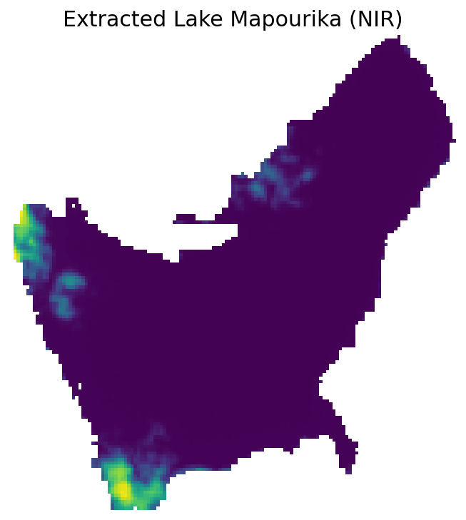
Output: Visual proof of the extraction. By converting the masked zeros to NaN, the area outside our vector boundary becomes completely transparent, leaving only the precise shape of the lake.
6. Summary
Effectively managing how data moves in and out of your computer’s memory is crucial for functional spatial programming.
Writing requires metadata: Arrays lack spatial context. Always copy the
.profilefrom the source image, update the data types if your math altered them, and pass those parameters into the write function.Respect memory limits: Satellite files are massive. Protect your system by reading only the specific bands you need, reducing data precision, or utilizing windowed reading.
Clip to save time: Subsetting arrays using array indices, geographic coordinates, or exact vector polygons (masks) restricts processing strictly to your area of interest.
Reproject to align: Use
rasterio.warpto resample and transform pixel grids to match local Coordinate Reference Systems (like moving from UTM to local standard projections).