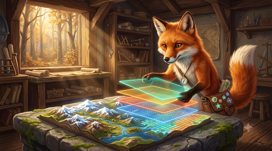
In the previous lessons, you learned how to wield GeoPandas to analyze discrete spatial shapes and how to use cartographic design to visualize them beautifully on interactive maps.
That was an essential step for mapping clear-cut features like roads, buildings, and political borders, but it raises a fundamental challenge:
What happens when the phenomenon you want to study does not have a clear boundary?
How do you draw a polygon around “temperature”? Where exactly does a mountain end and a valley begin? For these inherently fluid environmental variables, the discrete vector model breaks down.
This lesson introduces the other half of the spatial data science universe. Instead of placing isolated shapes onto an empty background, you will learn how to analyze the environment as a continuous surface using the Raster Data Model.
1. From discrete objects to continuous matrices
Programming raster analysis requires a massive shift in how you conceptualize space and compute data.
The raster model abandons the idea of empty space. It divides the entire world into a continuous, perfectly regular grid of cells (pixels), assigning a numerical value to every single location.
While this structure is beautifully simple, it introduces a massive computational challenge. A single modern satellite image can easily contain over 100 million individual pixels. If you attempted to process this data using the standard Python lists and for loops you learned earlier, your computer would hit a performance wall.
Therefore, you will transition your mental model from geographic geometries to multidimensional matrices. You will learn to bypass slow loops entirely by using the high-speed mathematical engine NumPy, alongside Rasterio, the industry-standard translator that bridges physical GeoTIFF files on your hard drive with lightning-fast arrays in your computer’s memory.
2. Why this matters for SDS
In spatial data science, the raster model is your window to Earth observation.
Without rasters, you are largely blind to the physical realities of the planet. Digital Elevation Models (DEMs), climate simulations, global precipitation records, and all satellite imagery are built on the raster data structure.
Mastering raster data allows you to answer continuous environmental questions: How steep is the slope of this specific valley? How much forest canopy was lost between 2019 and 2023? Where exactly are the new floodwaters from a breached dam settling?
By combining the spatial metadata management of Rasterio with the matrix mathematics of NumPy, you unlock Map Algebra. You will learn to add, subtract, and multiply millions of pixels simultaneously to extract hidden environmental signals—like moisture and snow cover—from the raw electromagnetic spectrum.
3. Learning objectives
After this lesson, you will be able to:
Shift to the continuous mental model Understand the raster data structure, the relationship between spatial resolution and pixel grids, and the performance limitations of standard Python.
Master the numerical engine Wield NumPy to slice, reshape, and filter multi-dimensional arrays, utilizing vectorization to execute instantaneous mathematical operations across millions of values.
Bridge files and memory Use Rasterio to safely read and write massive GeoTIFFs, securely managing the spatial metadata (Coordinate Reference Systems and Affine Transforms) that ties raw numbers to Earth.
Visualize environmental surfaces Translate raw numerical grids into interpretable spatial patterns by building RGB composites, stretching data histograms, and simulating 3D terrain with multidimensional hillshades.
Execute Map Algebra Derive complex environmental indices (like NDSI, EVI, and NDWI) and detect temporal landscape changes by calculating the spectral distance between perfectly aligned satellite bands.
Handle massive spatial data Actively manage your computer’s memory by reading chunks, modifying data types, clipping arrays to precise geographic vector boundaries, and reprojecting rasters safely.
4. Lesson structure
This lesson is structured to take you from the theoretical foundations of the grid to building custom satellite change-detection algorithms:
The Raster Model: Shifting paradigms from discrete geometries to continuous fields and the performance wall.
Crunching NumPy: Meeting the mathematical engine behind raster data and mastering multidimensional array manipulation.
Reading Spatial Grids: Using Rasterio to extract data from GeoTIFF files while preserving crucial spatial metadata.
Visualizing Raster Layers: Moving from quick previews to meaningful cartography with False Color Composites and terrain hillshades.
Map Algebra: Performing pixel-by-pixel mathematics to calculate environmental indices and spectral distance.
Data Handling: Managing memory, clipping rasters with vector polygons, reprojecting, and securely exporting your results.
Practical L9: Applying these skills to translate cloud-based algorithms into raw Python math to track the massive expansion of a global solar park.
5. Looking ahead
Lesson 9 is about the matrix.
You will learn not only how to open satellite imagery, but how to:
treat the environment as a continuous mathematical surface
apply complex linear algebra across millions of data points simultaneously
systematically combine discrete vector boundaries with continuous raster arrays
If Lesson 7 and 8 were about mapping boundaries, Lesson 9 is about analyzing every pixel within them.
The array manipulation and map algebra skills you build here are the absolute foundation of modern remote sensing and Earth observation. With both the Vector and Raster paradigms now under your belt, you possess a more complete core toolkit required to execute professional spatial data science workflows.