
In the previous chapters, you mastered the art of vector data. You learned how to represent the world using discrete geometries like points, lines, and polygons. You queried their intersections, measured their borders, and mapped their attributes.
But what happens when the phenomenon you want to study does not have a clear boundary?
How do you draw a polygon around “temperature”? Where exactly does a mountain end and a valley begin? For these inherently fluid environmental variables, the discrete vector model breaks down. To analyze the environment as a whole, we must shift our mental model from isolated shapes to continuous fields.
Chapter Relevance
Lab Relevance: ★★★ (Fundamental for all raster-based labs)
Project Relevance: ★★☆ (Crucial if your project incorporates environmental or satellite data)
Foundation: ★★★ (The absolute foundation for raster processing)
Time to Read: 10 minutes
In a nutshell: Learn how the raster data model represents continuous spatial phenomena using large numerical matrices, and why NumPy is required to process them.
Skip this if: You already deeply understand the difference between vector and raster data, and how geographic surfaces are stored as NumPy arrays.
1. Vectors vs. Rasters
There are two fundamental ways to conceptualize geographic space: discrete objects and continuous fields.
The vector model relies on the discrete object view. It assumes the world is largely empty, except where occupied by specific features with well defined boundaries. Think of a map of buildings or a network of roads. You can easily count them.
The raster model relies on the continuous field view. It assumes that for any given coordinate on Earth, a specific variable can be measured. Elevation, air pressure, soil moisture, and satellite imagery are continuous fields. In a raster, space is never empty. Even if a sensor fails to capture data for a specific location, the raster still records a specific “NoData” placeholder for that exact spot.
2. The Matrix
To represent these continuous fields digitally, the raster model divides space into an array of rectangular cells, commonly known as pixels.
You can visualize a raster layer as a massive two-dimensional spreadsheet or matrix. The physical size of each pixel on the ground determines the spatial resolution of the data. For example, in a 10-meter resolution satellite image, every single pixel represents a 10-by-10-meter square of the Earth’s surface.
Because the grid is perfectly uniform, a raster file does not need to store the exact latitude and longitude of every single pixel. It only needs to store the coordinates of the top left corner, the pixel size, and the massive grid of numbers. The computer can easily calculate the location of any other pixel based on its row and column position.
3. The Performance Wall
While the raster structure is beautifully simple, it introduces a massive computational challenge.
A standard regional digital elevation model or a single scene from a modern satellite can easily consist of 10,000 rows and 10,000 columns. That is 100 million individual pixels. If you attempted to store this data using standard nested Python lists and tried to multiply the values using a standard for loop, your computer would hit a performance wall. Standard Python is simply not optimized to iterate through millions of items one by one. The operation could take minutes or even hours to complete.
To perform spatial data science on continuous surfaces, we need a different engine.
4. Enter NumPy
The foundation of high-speed raster processing in Python is NumPy (numpy / Numerical Python). It is the core library for numerical computing and is used for representing and working with multidimensional arrays.
Instead of storing data in fragmented memory locations like standard lists, NumPy stores arrays in contiguous blocks of memory. More importantly, it utilizes a concept called vectorization. When you ask NumPy to multiply a raster grid by a constant, it does not loop through the pixels one by one. It pushes the operation down to highly optimized C code, performing the math on the entire matrix almost simultaneously.
This array architecture has a massive influence on how all modern raster libraries function. Whether you are using advanced tools like xarray or rasterio later in this course, under the hood, you are always manipulating a NumPy array.
Concept Check: The Loop Bottleneck
Scenario: You have a high-resolution satellite image with 10 million pixels representing land surface temperature. You want to convert the temperature from Kelvin to Celsius. Why shouldn’t you use a standard Python for loop to iterate through every pixel?
Option 1: for loops cannot access pixel values; you must use a spatial join.
Option 2: Standard Python lists and loops are not optimized for massive matrices and will hit a severe performance wall.
Option 3: The data is continuous, so you can only calculate the area, not the temperature.
Check your understanding
Answer: Option 2 Raster data relies on massive matrices. Standard Python loops iterate one by one, which takes far too long for millions of cells. NumPy solves this using ‘vectorization’, pushing operations down to optimized C code to compute the whole matrix almost instantly.
5. The Python Raster Ecosystem
While NumPy provides the raw mathematical power for representing and working with multidimensional arrays, writing raw matrix calculations to open a satellite image from scratch would be exhausting.
Because NumPy has a big influence on how other raster libraries function, the spatial data science community has built an entire ecosystem of specialized tools directly on top of it. There are a number of libraries widely used when working with raster data in Python.
Here are the core libraries you will encounter:
rasterio: This is the core library for working with GIS raster data. It acts as the fundamental bridge between Python and physical raster files on your hard drive.xarray: This library provides a user-friendly and intuitive way to work with multidimensional raster data that includes coordinates and attributes. You can think of it as the raster equivalent to GeoPandas, which is used for vector data processing.rioxarray: This is a powerful extension of therasteriolibrary that brings those same core functionalities directly on top of thexarraylibrary. It provides methods to conduct GIS-related operations with raster data, such as reading, writing, reprojecting, clipping, and resampling.xarray-spatial: Once your data is loaded and structured, this library provides methods for analyzing raster data. It includes advanced tools for focal and zonal operations, surface analysis, and pathfinding.geocube: This library provides methods for doing data conversions between raster and vector formats. It is the essential tool when you need to bridge the two mental models by rasterizing vector polygons or vectorizing raster pixels.
In addition to these foundational tools, there are a number of other libraries that are specialized to specific types of analyses or data. We will learn about a few of them later in the book. But for now, remember that whether you are calculating a vegetation index or reprojecting a digital elevation model, these libraries are all seamlessly passing NumPy matrices back and forth behind the scenes.
6. The Toy Terrain
To truly understand raster data, we need to strip away the geographic complexity and look at the raw numbers. To get a better sense of how raster data looks, we can start by creating a simple two dimensional array in Python using numpy.
We will modify this raster layer to represent a simple terrain that has a hill in the middle of the grid. We do this by setting higher numerical values in the center while the other values are represented with the value 0.
Step 1: The Empty Grid
Let us start by importing the numpy and matplotlib libraries which we use for calculating and visualizing our data.
Creating a simple 2D raster layer can be done easily by using the numpy method .zeros() which fills the cells (pixels) with zeros. Each zero represents a default pixel value, like an elevation of exactly 0 meters. You can think of this as an empty raster grid.
import numpy as np
import matplotlib.pyplot as plt

# Create a 5x5 array filled with zeros
raster_layer = np.zeros((5, 5))
print(raster_layer)
[[0. 0. 0. 0. 0.]
 [0. 0. 0. 0. 0.]
 [0. 0. 0. 0. 0.]
 [0. 0. 0. 0. 0.]
 [0. 0. 0. 0. 0.]]
Step 2: Sculpting the Terrain
Now we have a simple 2D array filled with zeros. Next, we modify the raster layer to represent a simple terrain and add larger numbers in the middle of the grid by setting higher values in the center.
We can do this by slicing the numpy array using the indices of the array and updating the numbers on those locations. Slicing numpy arrays happens in a similar manner as when working with standard Python lists. However, we do this in two dimensions by accessing the values stored in specific rows and columns.
Let us build the base of the hill (an elevation of 5) and the peak of the hill (an elevation of 10):
# Update a 3x3 block in the middle to have an elevation of 5
raster_layer[1:4, 1:4] = 5

# Update the exact center pixel to represent the peak with a value of 10
raster_layer[2, 2] = 10

print(raster_layer)
[[ 0.  0.  0.  0.  0.]
 [ 0.  5.  5.  5.  0.]
 [ 0.  5. 10.  5.  0.]
 [ 0.  5.  5.  5.  0.]
 [ 0.  0.  0.  0.  0.]]
Step 3: Visualizing the Matrix
As a result, we have a raster layer that simulates a simple terrain. We can also plot this raster layer using the matplotlib library and its .imshow() function that can be used to visualize arrays.
# Visualize the array
plt.imshow(raster_layer, cmap="terrain")

# Add cartographic context
plt.colorbar(label="Elevation")
plt.title("Simple Raster Layer representing a Hill")
plt.show()
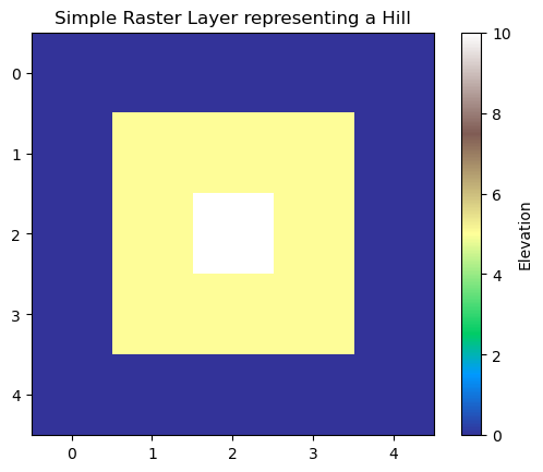
The colormap of the visualization was determined using the parameter cmap, while the plt.colorbar() function was used to add a legend to the right side of the image, and the plt.title() was used to add a simple title.
The Spatial Missing Link
This demonstrates a toy example of how we can produce a simple raster layer from scratch.
However, there are various aspects related to working with GIS raster data that we did not cover here. Basically, the data we have here is simply a two dimensional array (matrix) that does not tell anything about the spatial resolution of the data, the exact geographic coordinates, or the coordinate reference system this data is represented in.
Before we move on to real spatial data containing those missing elements, take a moment to explore the connection between raw numbers and topography. Below, you can interact with a numerical matrix to see exactly how changing the raw values of a grid instantly alters the physical topography and visual rendering of a continuous spatial field.
Interactive Explorer: Terrain Matrix Editor.
Change the numerical values inside the 5x5 matrix grid and watch how the rendered 3D terrain surface updates instantly. This demonstrates exactly how continuous geographic surfaces like elevation are stored and interpreted by the computer as a simple grid of numbers. For improved visibility of the explorer, follow this link.
7. Summary
The transition from vector to raster requires a shift in how you write code.
You are no longer extracting geometries and querying intersections. Instead, you are manipulating massive matrices of numbers. By leveraging the speed of multidimensional arrays, you can perform map algebra, overlay multiple spectral bands, and analyze continuous environmental phenomena across millions of pixels in milliseconds.