
Chapter Relevance
Lab Relevance: ★★★ (Essential for opening and manipulating time-series environmental data)
Project Relevance: ★★★ (Core to handling large climate and satellite data cubes)
Foundation: ★★★ (Fundamental shift from 2D raster logic to N-dimensional labels)
Time to Read: 15 minutes
In a nutshell: Learn how the xarray library organizes massive 3D+ environmental grids using human-readable dimension names instead of complex array indices.
Skip this if: You are already fully comfortable working with xarray.Dataset, xarray.DataArray, and label-based selection (.sel()).
In the previous lesson, you learned how to read spatial grids using Rasterio and process them using NumPy. That workflow is perfect for analyzing a single snapshot of the environment. However, Earth observation is fundamentally about change.
To analyze climate patterns, vegetation growth, or urban heat, you cannot look at one image. You need to process hundreds of repetitive observations simultaneously. This chapter introduces the Data cube Model, a conceptual shift that prepares you to handle massive, multidimensional environmental datasets using the xarray library.
1. Why xarray after Rasterio?
Rasterio is an excellent translator. It reads a GeoTIFF file from your hard drive and hands you a pure NumPy array. While NumPy is incredibly fast at math, it is completely blind to context.
If you load a massive climate dataset, NumPy might tell you the array shape is (2920, 25, 53). But that raw matrix does not tell you which axis is time, which axis is latitude, or what the units are. If you want to find the temperature for Zurich on July 1st, you have to mentally calculate the exact numeric index for that day, row, and column. This leads to code that is difficult to read and highly prone to silent errors.
The xarray library solves this exact problem. It brings the intuitive labeling power of Pandas directly into the multidimensional matrix operations of NumPy.
Just as geopandas makes tabular data spatially aware, a companion library called rioxarray provides robust GIS capabilities on top of xarray. Together, they allow you to read, project, and manipulate raster data using named dimensions (time, lat, lon) and coordinates, rather than raw numerical indices.
2. The third dimension and beyond
To understand xarray, you must shift your perspective from a flat map to a multidimensional cube.
A traditional satellite image or Digital Elevation Model exists in two spatial dimensions: X (longitude) and Y (latitude). Imagine taking a new satellite image of the exact same location every day for a year. If you physically stack these images on top of one another like pages in a book, the depth of that stack becomes a third dimension: Time.
The resulting structure is a Data Cube.
Within this cube, every single geographic pixel is no longer just a static value. If you select a specific coordinate and drill straight down through the layers of the cube, you extract a complete time series showing exactly how that location changed over the year.
However, environmental data cubes often go beyond just time. A single xarray object can align multiple components perfectly over the same geographic grid:
Spatial Dimensions: The X (longitude) and Y (latitude) axes.
Temporal Dimensions: The same raster repeated across days, months, or years.
Spectral Dimensions: Multiple sensor bands (Red, Green, Near-Infrared) stacked together.
Data Variables: Entirely different physical measurements (e.g., temperature, precipitation, and wind speed) sharing the exact same dimensions.
To visualize how a 2D grid transforms into a 3D time series, explore the interactive widget below.
Interactive Explorer: The Data Cube Model.
Click and drag to rotate the 3D model, and use the toggle button to switch between exploded and compact views of the temporal layers. Click any specific spatial pixel on the top grid to "drill down" through time, instantly extracting and plotting its 1D time series on the accompanying chart. This demonstrates exactly how multidimensional arrays store historical data for every single geographic location. For improved visibility of the explorer, follow this link.
3. DataArray and Dataset
When working with data cubes in Python, xarray provides two core data structures. Both of these build directly upon the logic of the pandas and geopandas libraries you have seen in previous lessons.
Understanding the relationship between these two structures is the foundation of multidimensional analysis.
The DataArray
A DataArray is a single labeled variable. You can think of it as the xarray equivalent of a pandas.Series, but designed to handle multidimensional raster matrices instead of flat columns.
Every DataArray consists of four key properties:
Values: The underlying NumPy array containing the raw numbers (e.g., the actual temperature readings).
Dimensions (dims): The named axes of the data (e.g.,
time,lat,lon).Coordinates (coords): The specific tick labels along those dimensions (e.g.,
2024-05-30, or47.3°N).Attributes (attrs): A dictionary holding arbitrary metadata (e.g., units, sensor type, or data source).
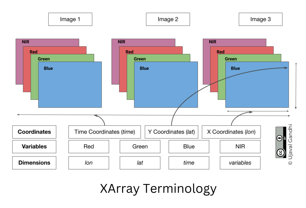
*A DataArray bundles the raw numerical data with named dimensions, coordinate labels, and metadata attributes. Source: SpatialThoughts*
The Dataset
A Dataset is a container that holds multiple DataArrays together.
In environmental science, you rarely measure just one variable. A weather model might predict temperature, precipitation, and wind speed simultaneously. A Dataset aligns all these different variables perfectly along the same shared coordinates.
You can think of a Dataset as the xarray equivalent of a geopandas.GeoDataFrame. Just as a GeoDataFrame stores multiple columns of data over the same exact geographic shapes, a Dataset stores multiple physical variables over the exact same multidimensional cube.
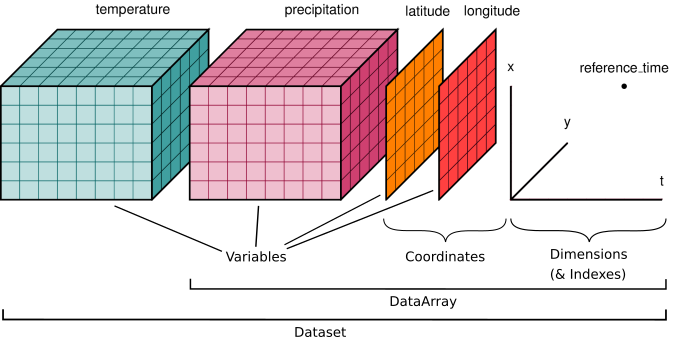
*A Dataset aligns multiple variables (DataArrays) inside a single container, sharing the exact same geographic and temporal dimensions. Source: xarray*
A first look in Python
The built in air_temperature tutorial dataset is a perfect way to see how this structure looks in practice.
When you open the file, xarray loads the entire container:
import xarray as xr

# Open the tutorial dataset container
ds = xr.tutorial.open_dataset("air_temperature")
ds
This object is a Dataset. In your Jupyter output, you will see it lists the dimensions (time, lat, lon), the coordinates, and a section called “Data variables”. Inside that data variables section, there is a single entry called air.
If you extract that specific variable using dictionary syntax, you pull out the DataArray:
# Extract the single variable from the container
air_temperature_array = ds["air"]
air_temperature_array
4. Why labels beat indices
The greatest advantage of the Data Cube model is that you stop writing code based on computer logic and start writing code based on human logic.
Under the hood, the values are still stored as a NumPy array. You can access that raw array with .values:
air_matrix = air_temperature_array.values
air_matrix.shape
(2920, 25, 53)If you work with this raw NumPy array directly, you must remember the meaning of every axis yourself.
# Pure NumPy: you must know that axis 0 is time, 1 is latitude, and 2 is longitude
temperature = air_matrix[100, 12, 20]
temperature
np.float64(274.7)That works, but it is fragile. The code no longer tells you what 100, 12, and 20 actually mean. You need to remember that:
100refers to the 101st time step12refers to the 13th latitude20refers to the 21st longitude
This is exactly the problem that xarray solves.
Positional selection with isel()
If you know the array positions but want your code to remain readable, use index selection with isel().
# Explicitly name the dimensions while still selecting by position
air_temperature_array.isel(time=100, lat=12, lon=20)
This is already safer than raw NumPy indexing because the dimension names make your intention clear.
You can also inspect which labels belong to that selected cell:
sample = air_temperature_array.isel(time=100, lat=12, lon=20)

print(sample)
print("Latitude:", float(sample["lat"]))
print("Longitude:", float(sample["lon"]))
print("Time:", str(sample["time"].values))
<xarray.DataArray 'air' ()> Size: 8B
array(274.7)
Coordinates:
    lat      float32 4B 45.0
    lon      float32 4B 250.0
    time     datetime64[ns] 8B 2013-01-26
Attributes:
    long_name:     4xDaily Air temperature at sigma level 995
    units:         degK
    precision:     2
    GRIB_id:       11
    GRIB_name:     TMP
    var_desc:      Air temperature
    dataset:       NMC Reanalysis
    level_desc:    Surface
    statistic:     Individual Obs
    parent_stat:   Other
    actual_range:  [185.16 322.1 ]
Latitude: 45.0
Longitude: 250.0
Time: 2013-01-26T00:00:00.000000000
Label selection with sel()
The real strength of xarray is label selection with sel(). Here you select values using meaningful coordinate labels instead of integer positions.
From the previous example, the selected cell corresponds to:
time = "2013-01-26T00:00:00.000000000"lat = 45.0lon = 250.0
Now you can select the exact same value again, but this time using the labels directly:
air_temperature_array.sel(time="2013-01-26T00:00:00.000000000", lat=45.0, lon=250.0)
This is much easier to read because the code itself now tells you what you selected:
the timestamp
2013-01-26the latitude
45.0the longitude
250.0
Instead of remembering array positions, you work directly with the labels that give the data meaning.
Concept Check: Positional vs. Label Selection
Scenario: You have a climate DataArray named precip with dimensions (time, lat, lon). You want to extract the precipitation data for the exact date “2024-01-01” at latitude 45.0 and longitude 10.0. Which command should you use?
A) precip.isel(time="2024-01-01", lat=45.0, lon=10.0)
B) precip.sel(time="2024-01-01", lat=45.0, lon=10.0)
C) precip[2024, 45, 10]
Check your understanding
Answer: B
The .sel() method is used for label-based selection, allowing you to pass the actual human-readable values (like dates and coordinates). The .isel() method is strictly for index-based positional selection, which requires raw integer array positions (like row 0, column 5).
Both values describe the same location on Earth. This is common in climate and Earth system datasets because it keeps longitude coordinates continuous across global grids.
5. Multidimensional data formats
xarray is domain agnostic. It acts as a universal translator that reads from and writes to a variety of scientific file formats. Because multidimensional environmental datasets are massive and often heterogeneous, these file formats use hierarchical structures—meaning they organize data into “groups” that act exactly like folders on your computer.
Depending on your project, you will encounter four major storage formats:
GeoTIFF and COG (
.tif): You already know GeoTIFFs from the previous lesson. They map perfectly to a singlexarray.Variable. However, TIFFs are inherently two dimensional per band. They have no native concept of a time axis or a vertical altitude axis. If you need 4D data, you must move beyond TIFFs. A Cloud Optimized GeoTIFF (COG) is a modern upgrade that allows you to stream specific geographic windows over the internet, whichxarrayhandles transparently.HDF5 (
.h5or.hdf5): The Hierarchical Data Format is a heavy duty, general purpose container for large scientific data. It behaves exactly like a UNIX filesystem. It contains “Groups” (folders), “Datasets” (multidimensional arrays), and “Attributes” (metadata). It supports advanced chunking and compression, making it a powerhouse for complex, nested data structures.NetCDF (
.nc): The classic standard in climate and oceanography. Interestingly, modern NetCDF4 is actually built directly on top of HDF5! It is an “opinionated subset” of HDF5 that enforces strict rules about how dimensions and coordinates must be defined. Because it requires explicit dimension scales, it maps perfectly to thexarrayDataset structure.Zarr (
.zarr): The modern format built for the cloud. While HDF5 and NetCDF are traditionally single massive files, Zarr stores data as a tree of groups holding arbitrary JSON metadata and thousands of tiny, separate chunked arrays. If you want to analyze a ten year temperature trend for one specific city, Zarr allowsxarrayto stream just the tiny chunks for that specific location directly from a remote server without downloading the rest of the globe.
6. Exercise: Thinking in cubes
Look again at the interactive cube visualizer and the examples in this chapter.
Your task:
Name three possible dimensions of an environmental data cube.
Explain the difference between a DataArray and a Dataset in one or two sentences.
Explain why label based selection is easier to read than pure NumPy indexing.
Give one example of a scientific question that requires a data cube instead of a single raster.
Sample solution
A good answer could be:
Three common dimensions are
time,lat, andlon. Other possible dimensions areband,x,y, orlevel.A
DataArraystores one labeled variable together with its dimensions, coordinates, and metadata. ADatasetis a container that stores multiple aligned DataArrays sharing the same coordinates.Label based selection is easier to read because it uses meaningful values such as dates and coordinates instead of raw integer positions.
A question such as “How did air temperature change at one location over two years?” requires a data cube because it needs repeated observations through time.
7. Summary
The Data Cube model is a structural paradigm that combines fast matrix operations with explicit spatial and temporal labels using the xarray library.
The Third Dimension: Adding dimensions (like time or altitude) transforms a static 2D raster into a dynamic, multidimensional data cube.
Core Structures: A
DataArrayholds a single variable and its labels (similar to apandas.Series), while aDatasetacts as a container for multiple perfectly aligned variables (similar to ageopandas.GeoDataFrame).Human Logic: Using label based selection (
.sel()) makes spatial querying intuitive, self documenting, and infinitely safer than guessing raw NumPy integer indices.Storage Formats: While
xarrayhandles the math in memory, it relies on advanced hierarchical and cloud optimized formats like GeoTIFF, HDF5, NetCDF, and Zarr to persistently store massive datasets on disk.
Now that you understand the underlying anatomy of a data cube, you are ready to learn how to actively slice, mask, and aggregate these multidimensional arrays in the next chapter.