
In the previous sections, we learned how to load shapes, project them onto a metric grid, and calculate their areas and buffers. However, we only manipulated one dataset at a time.
In this section, we transition to answering complex spatial questions by comparing two entirely different datasets. You will learn how to evaluate the physical relationships between geometries and use those relationships to filter data and find nearest neighbors.
1. Asking Spatial Questions
When we look at a map, our brains instantly recognize spatial relationships. We can easily see if a dot is inside a square or if two lines cross each other. Computers, however, only see lists of coordinates.
To teach the computer how to recognize these visual relationships, spatial data science uses Topological Spatial Relations. These are mathematical rules that describe how the interior, boundary, and exterior of two geometric shapes interact.
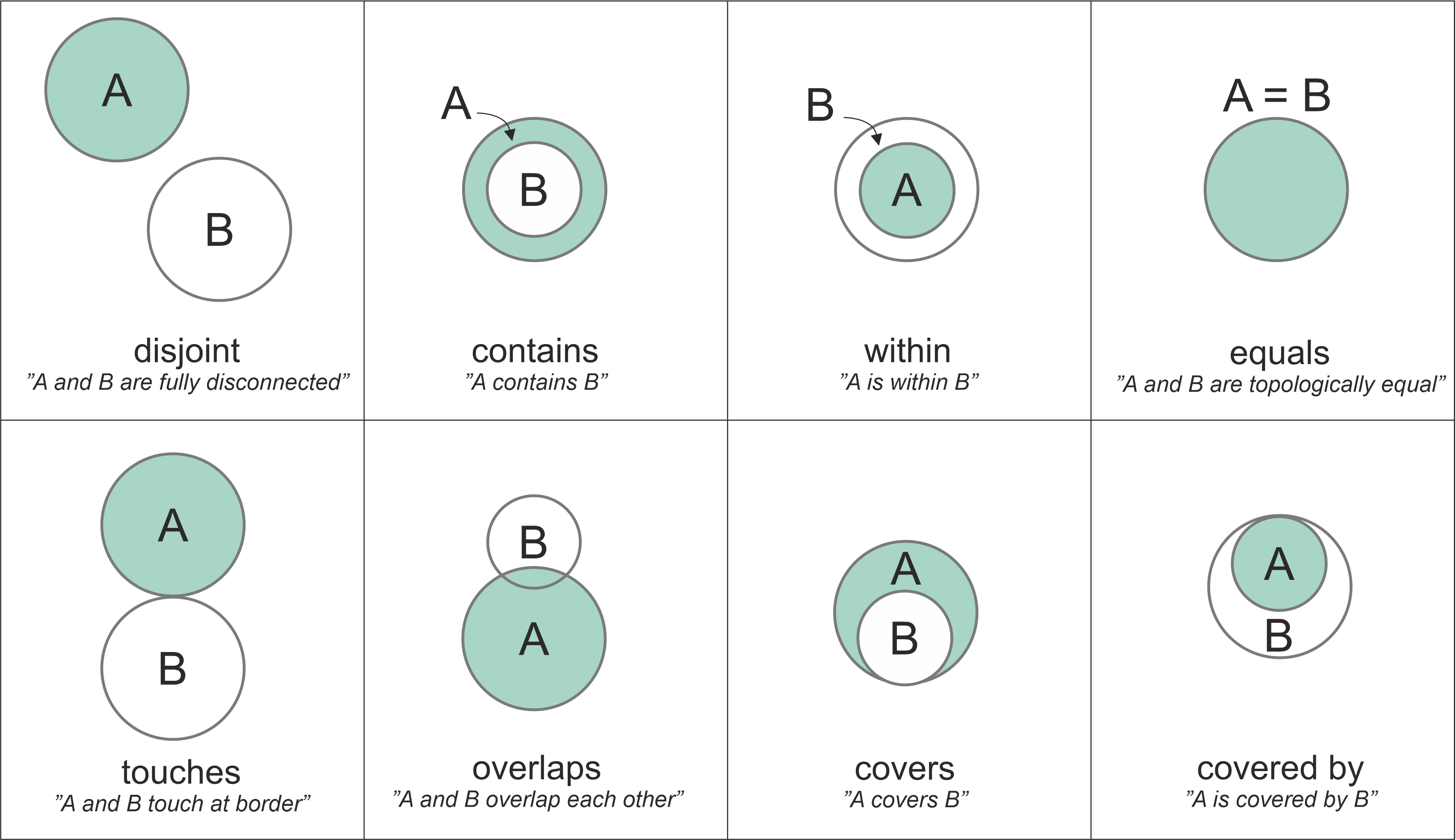
Common topological relationships. Notice how the mathematical definitions rely strictly on how the interiors and borders of the two shapes interact. Modified after Egenhofer et al. (1992). Source: Geopython
When you ask GeoPandas a spatial question (e.g., “Are these two shapes touching?”), it evaluates these mathematical rules under the hood and returns a simple Boolean answer: True or False. We refer to these evaluation methods as spatial predicates.
While there are many possible mathematical combinations, GeoPandas provides 10 core methods to test these relationships.
The Core Three
You will use these three spatial predicates for the vast majority of your spatial queries:
.intersects(): ReturnsTrueif the geometries share at least one point in common. This is the broadest and most commonly used query. (If a shape touches, crosses, or is within another shape, it also intersects it)..within(): ReturnsTrueif geometry A is completely inside the boundary of geometry B..contains(): ReturnsTrueif geometry A completely encloses geometry B. (This is the exact inverse of.within()).
Other Useful Predicates
Depending on the specific rules of your analysis, you might need more precise constraints:
.disjoint(): ReturnsTrueif the geometries are completely separated. (The exact opposite of.intersects())..touches(): ReturnsTrueif the geometries share a border/edge, but their interiors do not overlap at all..overlaps(): ReturnsTrueif the geometries’ interiors intersect partially, but neither is completely inside the other..equals(): ReturnsTrueif both geometries are topologically perfectly identical..crosses(): ReturnsTrueif the geometries intersect, but their intersection creates a shape of a lower dimension (e.g., a line crossing a polygon creates a line, not a polygon)..covers()/.covered_by(): Very similar to contains and within, but slightly more lenient because they allow the shapes to share exact boundaries.
2. Intersects, Contains, and Within
Let us test these core relationship methods using two distinct datasets: the polygonal borders of the Swiss cantons, and the point coordinates of the MeteoSwiss pollen monitoring stations.
First, we will load both datasets, ensure they share the exact same Coordinate Reference System (EPSG:2056), and extract a single canton and a single station to compare.
import geopandas as gpd
import pandas as pd
import numpy as np

# 1. Load the Cantons Polygons
cantons_gdf = gpd.read_file("swissBoundaries3D_cantons.gpkg")

# Extract just the geometry for the canton of Zurich
canton_zh = cantons_gdf[cantons_gdf["name"] == "Zürich"].geometry.iloc[0]

# 2. Load the Pollen Stations Points (CSV -> GeoDataFrame)
pollen_df = pd.read_csv("meteoswiss_pollen_network.csv")
pollen_gdf = gpd.GeoDataFrame(
    pollen_df, geometry=gpd.points_from_xy(pollen_df.X, pollen_df.Y), crs="EPSG:2056"
)

# Extract just the geometry for the specific station located in Zurich
station_zh = pollen_gdf[pollen_gdf["station_name"] == "Zürich"].geometry.iloc[0]
The Geometry Methods
Because canton_zh is a Shapely Polygon and station_zh is a Shapely Point, they possess built-in methods to test their relationships against one another.
To understand how these methods work, we must test them in both directions. Does the order in which we ask the question matter? Let us ask the computer six specific questions:
# 1. Testing 'Contains' (Does the first shape completely enclose the second?)
print("Canton contains station:", canton_zh.contains(station_zh))
print("Station contains canton:", station_zh.contains(canton_zh))

# 2. Testing 'Within' (Is the first shape completely inside the second?)
print("\nStation within canton:", station_zh.within(canton_zh))
print("Canton within station:", canton_zh.within(station_zh))

# 3. Testing 'Intersects' (Do the two shapes share ANY space at all?)
print("\nStation intersects canton:", station_zh.intersects(canton_zh))
print("Canton intersects station:", canton_zh.intersects(station_zh))
Output:
Canton contains station: True
Station contains canton: False

Station within canton: True
Canton within station: False

Station intersects canton: True
Canton intersects station: True
This output reveals a critical rule of spatial querying: Order matters immensely for most predicates! * Asymmetric Methods: .contains() and .within() are directional. A massive polygon can contain a tiny coordinate point, but a point can never contain a polygon. Notice, however, that they are perfect inverse methods of each other. Use whichever makes your code read more naturally.
Symmetric Methods:
.intersects()is bi-directional. If shape A touches shape B, then shape B must be touching shape A. The order does not matter.
Concept Check: The Rhine River
You have a LineString geometry representing the entire Rhine River (flowing from the Swiss Alps all the way to the Netherlands) and a Polygon geometry representing the country of Switzerland (swiss_poly).
Based on the mathematical rules of spatial predicates, which of the following queries will return True?
A) rhine_line.within(swiss_poly)
B) swiss_poly.within(rhine_line)
C) swiss_poly.contains(rhine_line)
D) rhine_line.intersects(swiss_poly)
Check your understanding
Answer: D
Because the Rhine River extends geographically beyond Switzerland’s borders into Germany and the Netherlands, it is not completely .within() the country (A is False), nor does Switzerland completely .contains() it (C is False). Furthermore, a massive 2D country polygon can never be .within() a 1D river line (B is False). The only topologically true statement is that they share geographic space along the way, meaning they .intersects() (D is True).
Scaling Up: The Spatial Loop
Checking one station against one canton is easy. But what if we want to calculate a brand new regional metric for our dataset?
For this example, we will calculate the average altitude of the pollen stations inside each individual canton. (You can imagine altitude here as a tangible substitute for any real-world scientific measurement you might want to aggregate, such as daily pollen concentrations, temperature, or rainfall!)
To do this, we can loop through every single canton and ask the computer to find which stations fall .within() its borders. If it finds any, we will calculate their average altitude and save it directly into the cantons_gdf attribute table.
import numpy as np
import matplotlib.pyplot as plt

# Create a new empty column filled with NaN (Not a Number)
cantons_gdf["avg_pollen_alt"] = np.nan

# Loop through each row in the cantons dataset
for idx, canton_row in cantons_gdf.iterrows():
    # Grab the current canton's polygon
    canton_geom = canton_row.geometry

    # Ask the question: Which stations are WITHIN this specific canton?
    # This creates a True/False mask to filter the stations!
    stations_inside = pollen_gdf[pollen_gdf.geometry.within(canton_geom)]

    # If the canton actually contains one or more stations...
    if not stations_inside.empty:
        # Calculate the mean altitude of those specific stations
        avg_alt = stations_inside["altitude"].mean()

        # Save the result into our new column for this specific canton
        cantons_gdf.at[idx, "avg_pollen_alt"] = avg_alt

# Let's filter out the NaNs and look at the cantons that actually have stations
has_stations = cantons_gdf.dropna(subset=["avg_pollen_alt"])
print("Cantons with stations and their average altitude:")
display(has_stations[["name", "avg_pollen_alt"]].head().round(1))

# Let's visualize our brand new metric!
# We use 'missing_kwds' to color the cantons that didn't have any stations in light grey
ax = cantons_gdf.plot(
    column="avg_pollen_alt",
    cmap="viridis",
    legend=True,
    legend_kwds={"label": "Average Station Altitude (m)"},
    missing_kwds={"color": "lightgrey", "label": "No Stations"},
    figsize=(10, 6),
    edgecolor="white",
)
ax.set_title("Average Altitude of Pollen Stations per Canton")
ax.axis("off")
plt.show()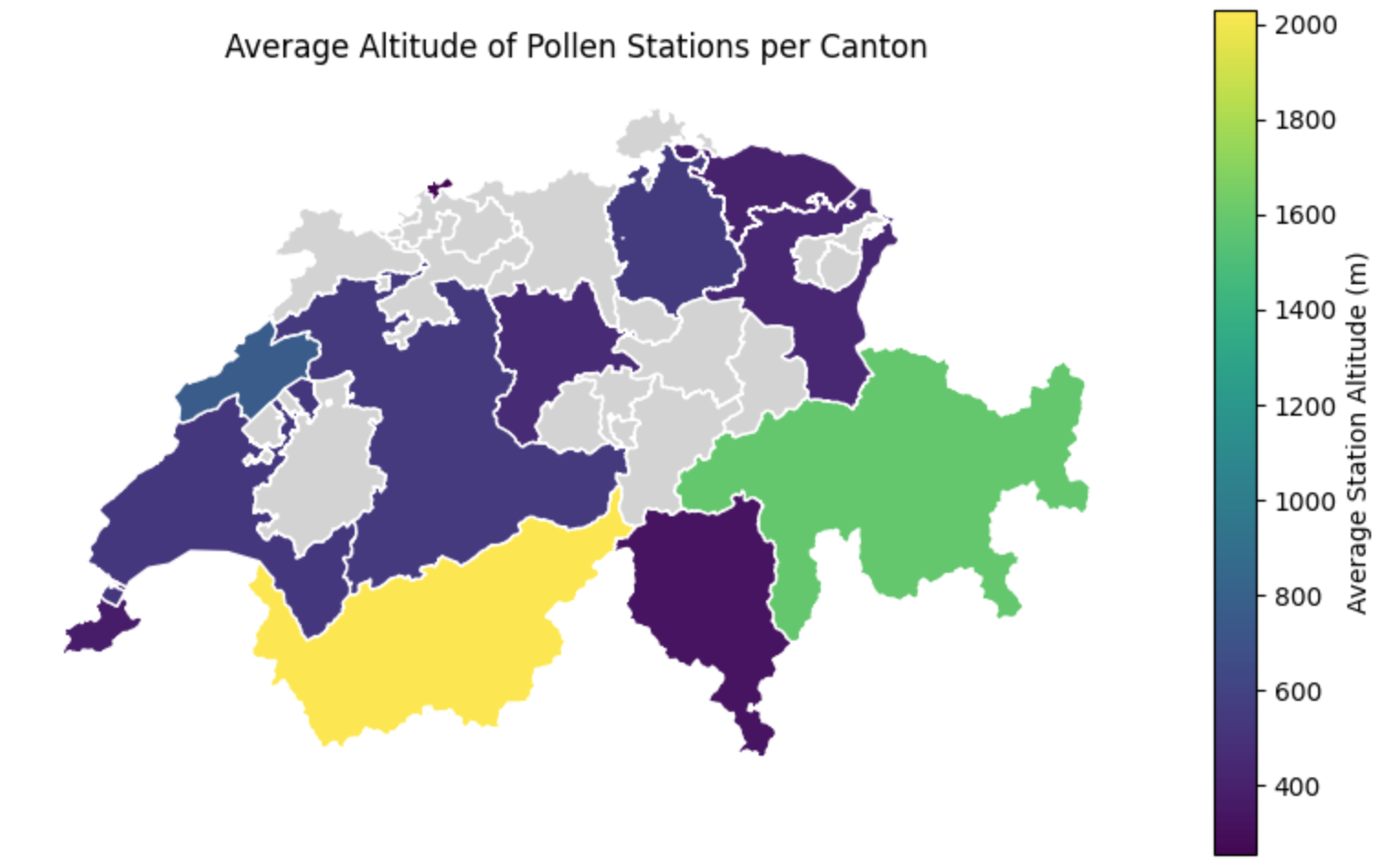
Visualizing our engineered metric. By combining a simple Python loop with a spatial predicate (.within()), we successfully generated a brand new geographical layer. Notice how the light grey cantons were automatically skipped by our if not stations_inside.empty: logic!
3. Filtering by Location
In the previous section, we used a for loop to test geometries one by one. While loops are useful, they are very slow for large datasets. The true power of GeoPandas shines when we apply spatial predicates to entire DataFrames at once.
In early chapters, you learned how to filter Pandas DataFrames using logical conditions (e.g., data[data["population"] > 1000]). In GeoPandas, you can use geography itself as the logical condition!
Let us answer a critical safety question: If a nuclear emergency required a 16 km evacuation zone around the Beznau nuclear power plant, how many primary homes in the surrounding communes would be affected?
We will load the Swiss housing inventory (which contains communal polygons and household counts in a column called ZWG_3010) and the Nuclear Power Plant dataset.
# 1. Load the Housing Inventory (Communal polygons)
housing_gdf = gpd.read_file("wohnungsinventar.gpkg")

# 2. Load the Nuclear Power Plants and isolate Beznau
npp_df = pd.read_csv("NuclearPowerPlant.csv")
npp_gdf = gpd.GeoDataFrame(
    npp_df, geometry=gpd.points_from_xy(npp_df.X, npp_df.Y), crs="EPSG:2056"
)
beznau = npp_gdf[npp_gdf["Name"] == "Kernkraftwerk Beznau"].geometry.iloc[0]

# 3. Create the 16km (16,000m) Evacuation Buffer around Beznau
evac_zone = beznau.buffer(16000)
Now, instead of writing a loop, we will ask the entire housing_gdf dataset which communal polygons intersect with our evacuation zone. This generates a Boolean mask—a simple list of True and False values—which we can use to instantly filter the rows!
# 4. Create a Boolean mask using a spatial predicate
in_danger_mask = housing_gdf.geometry.intersects(evac_zone)

# Let's peek at the mask to see what it looks like:
print("The Boolean Mask:")
print(in_danger_mask.head())

# 5. Filter the GeoDataFrame using the mask (Keep only the True rows)
impacted_communes = housing_gdf[in_danger_mask]

# 6. Sum the primary homes from the filtered dataset (ZWG_3010 = Number of primary homes)
total_impacted_homes = impacted_communes["ZWG_3010"].sum()

print(f"\nTotal primary homes impacted: {total_impacted_homes:,}")
With just two lines of spatial filtering logic, we instantly calculated demographic vulnerability based purely on geographic location!
To prove that our spatial filter worked perfectly, let us visualize the results. We will plot all the communes in light grey, overlay our filtered impacted_communes in red, and draw the 16km evac_zone boundary on top.
import matplotlib.pyplot as plt

fig, ax = plt.subplots(figsize=(10, 6))

# Plot the base map of all communes
housing_gdf.plot(ax=ax, color="whitesmoke", edgecolor="lightgrey")
# Plot ONLY the filtered communes that intersected the zone
impacted_communes.plot(ax=ax, color="lightcoral", edgecolor="darkred")
# Plot the 16km evacuation zone outline and the Beznau point
gpd.GeoSeries([evac_zone]).plot(
    ax=ax, facecolor="none", edgecolor="black", linewidth=2, linestyle="--"
)
gpd.GeoSeries([beznau]).plot(ax=ax, color="black", marker="*", markersize=100)
# Zoom into the relevant area
ax.set_xlim(2630000, 2690000)
ax.set_ylim(1250000, 1290000)
ax.set_title("Swiss Communes Impacted by Beznau 16km Evacuation Zone")
ax.axis("off")
plt.show()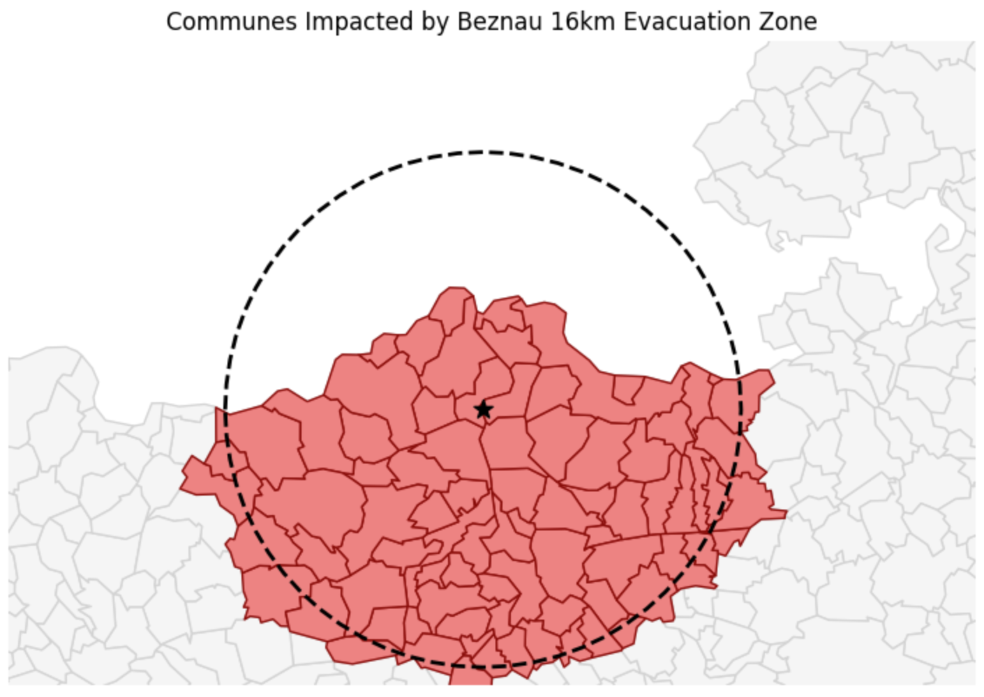
Visual proof of our spatial filter. Notice that if even a tiny sliver of a commune’s border crossed into the dashed 16km evacuation zone, the entire commune polygon was correctly flagged as True by the .intersects() predicate and highlighted in red.
4. Nearest Neighbor
Sometimes geometries do not touch or overlap at all, but you still need to know their spatial relationship. A common task is finding the absolute closest feature between two different datasets.
Instead of writing complex mathematical loops to calculate the distance between every single point, GeoPandas provides the incredibly fast .sjoin_nearest() method (Spatial Join Nearest). It calculates the distance from every geometry in your primary dataset to the geometries in a secondary dataset, and immediately joins the attribute data of the closest match.
Let us find the closest hospital landing site for every Swiss Alpine Club (SAC) mountain hut in case of a helicopter medical emergency.
import geopandas as gpd

# 1. Load both datasets
# (Both files are already in the Swiss metric grid, but adding .to_crs()
# right when you load data is a fantastic safety habit to prevent degree-errors!)
huts_gdf = gpd.read_file("alpine_huts.gpkg").to_crs(epsg=2056)
hospitals_gdf = gpd.read_file("hospital_landing_sites.geojson").to_crs(epsg=2056)

# 2. Find the nearest hospital for every hut
# - how="left": Keep all the huts in our results, even if something goes wrong.
# - distance_col="distance_m": Automatically record the exact distance in meters.
emergency_plan = huts_gdf.sjoin_nearest(
    hospitals_gdf, how="left", distance_col="distance_m"
)

# 3. View the results (Showing the Hut Name, the Closest Hospital, and the Distance)
display(emergency_plan[["name_left", "name_right", "distance_m"]].head(3).round(1))Output:
| name_left | name_right | distance_m | |
|---|---|---|---|
| 0 | Mischabelhütte | Visp Spital | 19826.8 |
| 1 | Rifugio Sant’Anna | Locarno Clinica Santa Chiara | 6983.1 |
| 2 | Capanna Piandios | Acquarossa Ospedale | 5338.4 |
This operation requires a massive amount of background math, but thanks to advanced spatial indexing (KD Trees) working under the hood, GeoPandas can cross-reference and match thousands of points in milliseconds.
Visualizing the Connections
To truly understand what the computer just did, we can draw a map that explicitly connects every mountain hut to its newly assigned hospital.
Do not worry about the plotting syntax right now! We will formally introduce advanced mapping (matplotlib) in the next session. Treat this as an optional “sneak peek” into what you will be able to do next week.
To draw these connecting lines, we use the index_right column (which .sjoin_nearest() automatically creates to remember which hospital it matched with) to retrieve the exact hospital coordinates.
from shapely.geometry import LineString
import matplotlib.pyplot as plt

# 1. Bring the hospital's geometry back into our results table
emergency_plan = emergency_plan.merge(
    hospitals_gdf[["geometry"]],
    left_on="index_right",
    right_index=True,
    suffixes=("", "_hospital")
)

# 2. Create a brand new "flight path" line connecting the hut to the hospital
emergency_plan["flight_path"] = emergency_plan.apply(
    lambda row: LineString([row["geometry"], row["geometry_hospital"]]), axis=1
)

# 3. Tell GeoPandas to use our new flight paths as the active geometry for plotting
flight_paths_gdf = emergency_plan.set_geometry("flight_path")

# 4. Plot the results!
fig, ax = plt.subplots(figsize=(10, 6))

# Plot the flight paths in grey
flight_paths_gdf.plot(ax=ax, color="grey", linewidth=0.5, linestyle="--");

# Plot the huts as blue triangles
huts_gdf.plot(ax=ax, color="blue", marker="^", markersize=15, label="SAC Huts");

# Plot the hospitals as red crosses
hospitals_gdf.plot(ax=ax, color="red", marker="+", markersize=60, label="Hospitals");

ax.set_title("Emergency Helicopter Flight Paths (Nearest Hospital)")
ax.axis("off")
plt.legend()
plt.show()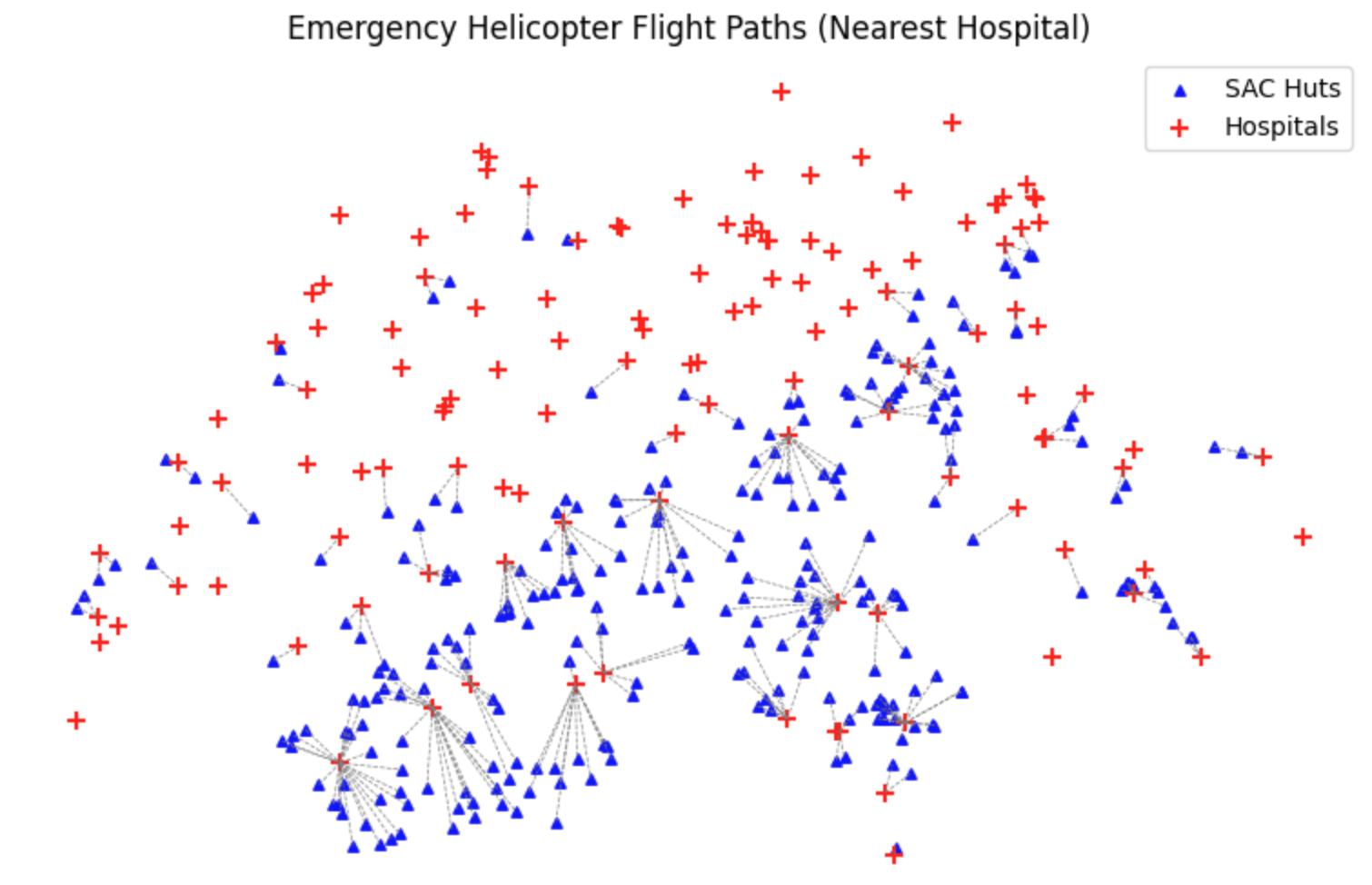
Visual proof of our .sjoin_nearest() calculation. The dashed lines represent the shortest possible flight path from each mountain hut to its assigned medical facility.
Advanced Tip: Search Limits
Helicopters have limited fuel, and in medical emergencies, time is critical. Look at the Mischabelhütte in the output above—it is almost 20 kilometers away from the nearest hospital! What if a rescue company only wants to find hospitals that are within a strict 15-kilometer flight radius?
You can make your nearest neighbor search even faster by passing the max_distance parameter:
# Only find hospitals if they are within 15,000 meters
emergency_plan = huts_gdf.sjoin_nearest(
    hospitals_gdf,
    distance_col="distance_m",
    max_distance=15000
)
(Note: If you ran this code, the Mischabelhütte would simply be dropped from the final results, as it has no hospitals within that 15km search radius!)
5. Exercise: Point in Polygon
It is time to test your spatial querying skills. We have GPS tracking data from wolves across Switzerland, but we are only interested in studying their movements when they are safely inside protected national park boundaries.
Your task is to use a spatial predicate as a Boolean mask to filter the GPS tracks.
Tasks:
Load Data: Load the two datasets and ensure both are in
EPSG:2056.Real-World Tip: Both of these files actually contain multiple spatial layers! To suppress GeoPandas’ warnings, you must specify exactly which layer to open. Use
layer="Schneeschuhwanderwege"for the wolf tracks (apparently our wolves like to follow the snowshoe trails!), andlayer="N2026_Revision_Park_20250430"for the parks.
Merge Parks: The parks dataset contains dozens of individual polygons. To make our query faster, merge them into a single massive “protected zone” geometry using
all_parks = parks_gdf.geometry.union_all().Filter by Location: Create a Boolean mask by checking which geometries in your wolf tracks dataset are
.within()theall_parksgeometry.Apply Mask: Filter the wolf GeoDataFrame using your mask to create a new variable called
protected_wolves.Count: Use
len()to see how many GPS tracks fell entirely inside the park boundaries compared to the original dataset.
# Write your code here
Sample solution
import geopandas as gpd

# 1. Load Data (Specifying the exact layer prevents warnings!)
wolves_gdf = gpd.read_file("wolf_tracks_switzerland.gpkg", layer="Schneeschuhwanderwege").to_crs(epsg=2056)
parks_gdf = gpd.read_file("swiss_parks.shp.zip", layer="N2026_Revision_Park_20250430").to_crs(epsg=2056)

# 2. Merge Parks into a single massive geometry
all_parks = parks_gdf.geometry.union_all()

# 3. Create the spatial boolean mask
inside_park_mask = wolves_gdf.geometry.within(all_parks)

# 4. Filter the dataframe using the mask
protected_wolves = wolves_gdf[inside_park_mask]

# 5. Print counts
print(f"Original GPS tracks: {len(wolves_gdf)}")
print(f"Tracks strictly inside parks: {len(protected_wolves)}")

# Optional Plotting
ax = parks_gdf.plot(color="lightgreen", edgecolor="darkgreen", figsize=(10, 6));
wolves_gdf.plot(ax=ax, color="lightgrey", markersize=1, alpha=0.5);
protected_wolves.plot(ax=ax, color="red", markersize=5);
ax.set_title("Wolf Tracks Inside Swiss National Parks")
ax.axis("off")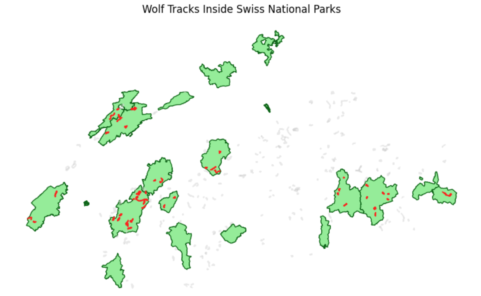
Applying a Point-in-Polygon (or Line-in-Polygon) spatial query. Because we used .within(), only the tracks that are completely inside the protected park boundaries are selected and highlighted in red.
6. Summary: Spatial Querying
In this section, you unlocked the ability to link disparate datasets together purely based on where they exist in the real world. From calculating nuclear evacuation zones to routing emergency helicopters and tracking wolves, you have learned the foundational logic of all advanced geographic information systems.
Key takeaways
Topological Rules: Spatial predicates are mathematical evaluations that return
TrueorFalsedepending on how shapes physically interact (or don’t).The Core Three: Memorize
.intersects(),.contains(), and.within(). They are your primary tools for querying space. Always remember that order matters when using asymmetric predicates like contains and within!Geographic Filtering: Just like filtering text or numbers in standard Pandas, you can use a spatial predicate to generate a Boolean mask and filter an entire GeoDataFrame at once—no slow
forloops required.Nearest Neighbor: When items do not touch, use
.sjoin_nearest()to rapidly calculate the closest feature between two datasets and merge their attributes. Remember to usemax_distanceto set logical real-world limits (like maximum flight ranges) and speed up your code.
What comes next?
We have successfully used spatial relationships to filter data (e.g., keeping only the wolves inside the park). But what if we want to permanently merge the columns of two overlapping datasets together?
In the final section of this chapter, Spatial Joins, we will explore how to fuse datasets based on their spatial relationships to create entirely new, multi-dimensional analytical tables!