
In the previous section, we successfully loaded and plotted geographic shapes. However, we ignored a critical question: how does the computer know exactly where on the planet those shapes belong?
This section addresses the most common source of frustration in Geographic Information Systems (GIS): Projections. You will learn why mapping the Earth is mathematically complicated, how to identify your current coordinate system, and how to safely manipulate it using GeoPandas.
Before we begin, please download the global administrative boundaries dataset provided by Natural Earth.
1. What is a CRS?
A Coordinate Reference System (CRS) is the mathematical framework that links the coordinates in your dataset to actual, physical locations on Earth. Without a CRS, your data is just a floating collection of arbitrary shapes.
There is a fundamental problem in spatial science: The Earth is a 3D curved surface, but our screens and paper maps are 2D and flat.
To understand this, think of the classic “Orange Peel Analogy.” Imagine trying to peel an orange and flatten the skin completely perfectly onto a table. You cannot do it without tearing, stretching, or squashing the peel.
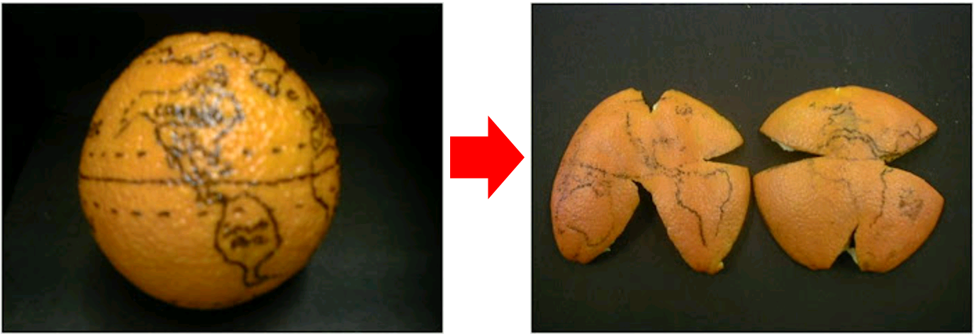
The Orange Peel Analogy. Flattening a 3D sphere inevitably results in tearing, stretching, or distortion. Map projections are mathematical attempts to control exactly where and how this distortion occurs. Source: Geopython
Because of this, there are two distinct families of Coordinate Reference Systems:
Geographic Coordinate Systems (The 3D Globe)
A geographic CRS treats the Earth as a 3D sphere (or more accurately, an ellipsoid). Locations are measured using angles from the center of the Earth.
Units: Degrees (Latitude and Longitude).
Pros: Exact global positioning. Excellent for storing raw GPS data.
Cons: You cannot easily calculate accurate physical distances (like meters) or areas. Because the Earth is a sphere, the physical distance between lines of longitude actively shrinks as you move from the equator toward the poles.
Projected Coordinate Systems (The 2D Map)
A projected CRS applies a mathematical formula (a “map projection”) to flatten the 3D globe onto a 2D Cartesian plane (an X and Y grid).
Units: Metric measurements (typically Meters).
Pros: Perfect for accurately calculating real-world areas, lengths, and distances.
Cons: Because flattening the orange peel always causes distortion, every projection must sacrifice some accuracy. Depending on the math used, a projection might preserve Shapes (Conformal), Areas (Equal Area), or Distances (Equidistant), but never all three at once.
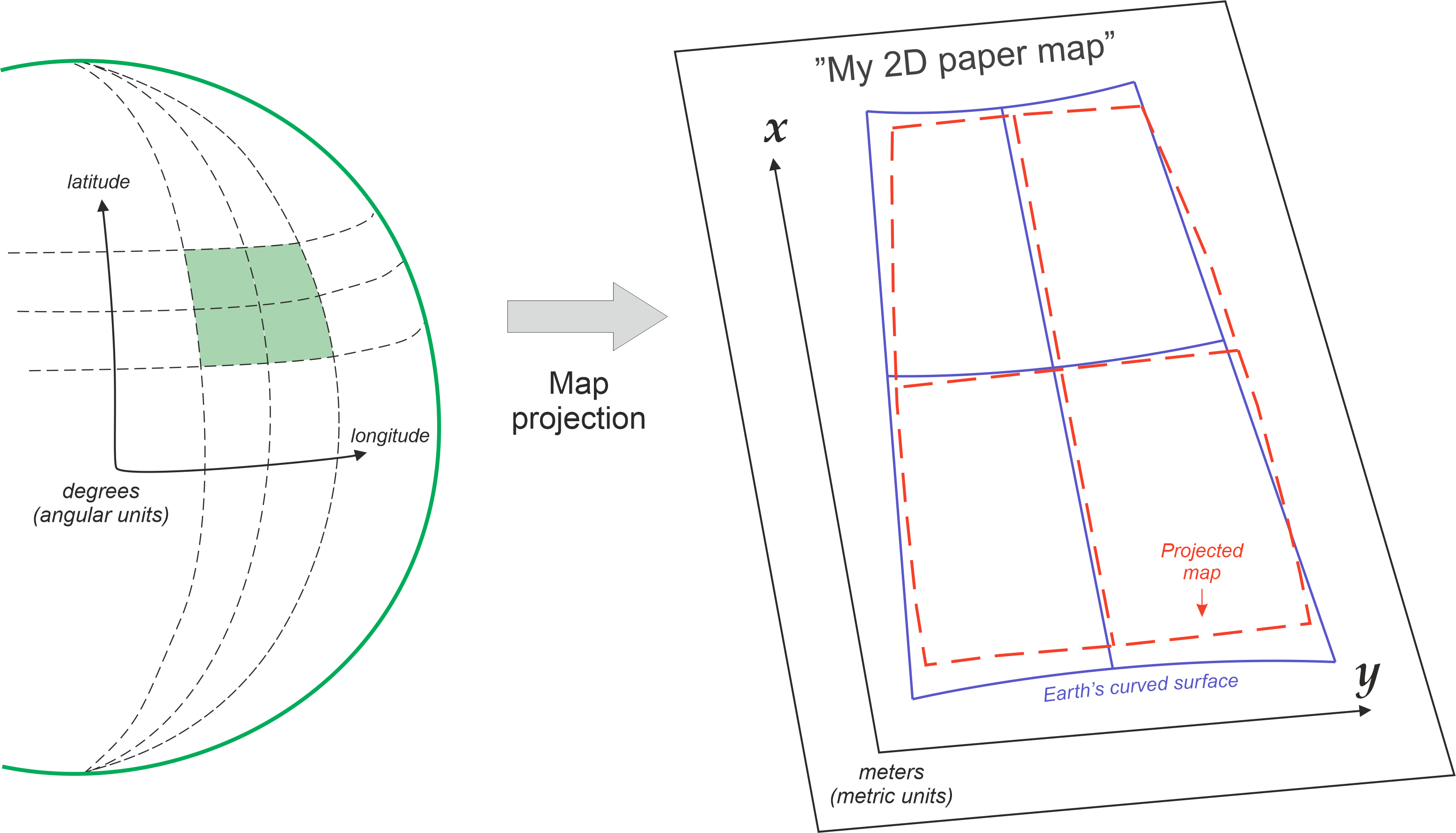
The conceptual transition from a 3D Geographic Coordinate System (measured in angular degrees) to a 2D Projected Coordinate System (measured in metric distances on a Cartesian grid). Source: Geopython
2. Checking and Parsing the CRS (.crs)
Whenever you load a new spatial dataset, the very first thing you should do after looking at .head() is check its Coordinate Reference System.
Let us load our global countries dataset and inspect its spatial reference using the .crs attribute.
import geopandas as gpd

# Load the global countries dataset directly from the zip archive
world_gdf = gpd.read_file("ne_50m_admin_0_countries.zip")

# Inspect the Coordinate Reference System
print(world_gdf.crs)
Output:
EPSG:4326That short EPSG:4326 output is incredibly important! It tells GeoPandas exactly what mathematical grid our geometries are drawn on.
But GeoPandas is actually hiding a lot of powerful information here. Under the hood, .crs returns a rich spatial object powered by a library called pyproj. We can actually ask this object for specific, human-readable details about our grid:
# Extracting specific characteristics from the CRS object
print("Name of the CRS:", world_gdf.crs.name)
print("Is it geographic (degrees)?", world_gdf.crs.is_geographic)
print("Is it projected (meters)?", world_gdf.crs.is_projected)
Output:
Name of the CRS: WGS 84
Is it geographic (degrees)? True
Is it projected (meters)? False
Defining a Missing CRS (.set_crs)
Sometimes, you will load a file and print(gdf.crs) will output None. This means the creator of the data was sloppy and forgot to include the spatial metadata!
When this happens, GeoPandas will still load the geographic shapes, but it will refuse to do any spatial math or map projections because it doesn’t know what grid the numbers belong to.
To fix this, you must manually assign the correct CRS using the .set_crs() method. Because our coordinates are clearly in degrees (longitude/latitude), we know the missing grid is WGS84 (EPSG 4326):
# How to manually define a CRS if your dataset is missing one
# (Note: This does not change the math/coordinates, it just adds the missing label!)
world_gdf = world_gdf.set_crs(epsg=4326)3. EPSG Codes Explained
Spatial metadata can be long and complex (sometimes requiring dozens of lines of text to describe the exact mathematical formulas of the ellipsoid). To make life easier, the spatial data community uses the EPSG Registry (originally created by the European Petroleum Survey Group).
EPSG codes are simple 4- to 5-digit numbers that act as a universal shorthand for specific coordinate systems. Instead of memorizing complex mathematical parameters, you only need to know a few key codes.
Here is your essential cheat sheet for the most important EPSG codes in European and global spatial data:
Essential EPSG Codes
| EPSG Code | Type | Name | Best Used For |
|---|---|---|---|
| 4326 | Geographic (Degrees) | WGS 84 | The global standard for GPS coordinates and raw latitude/longitude data. |
| 3857 | Projected (Meters) | Web Mercator | The standard for Google Maps and interactive web maps. (Distorts area heavily towards the poles!) |
| 8857 | Projected (Meters) | Equal Earth | Global maps where preserving accurate surface area sizes is important. |
| 3035 | Projected (Meters) | ETRS89 / LAEA | Statistical analysis and mapping across the entire continent of Europe. |
| 2056 | Projected (Meters) | CH1903+ / LV95 | The official highly accurate local projection for Switzerland. |
| 32632 | Projected (Meters) | UTM Zone 32N | A highly accurate metric zone covering parts of Switzerland and central Europe. |
Looking back at our .crs output, we see our world_gdf is using EPSG:4326. This means our dataset is currently unprojected, utilizing degrees of longitude and latitude. If we want to accurately calculate the physical area of these countries in square kilometers, we are going to have to change that!
Concept Check: Choosing the Right EPSG
You are tasked with calculating the exact area (in square kilometers) of all the national parks in Switzerland to see if they meet environmental protection quotas.
Based on the cheat sheet above, which EPSG code should you transform your data into before doing the math?
A) EPSG 4326 (WGS 84)
B) EPSG 3857 (Web Mercator)
C) EPSG 2056 (CH1903+ / LV95)
Check your understanding
Answer: C You need a Projected (Metric) CRS to calculate area, which immediately eliminates A. While B is projected, Web Mercator heavily distorts area. C (EPSG 2056) is the official, highly accurate local metric projection for Switzerland and will give you the most exact square kilometer calculations.
4. Reprojecting Data (.to_crs)
If your data is in degrees (EPSG:4326), but you want to calculate the area of a country in square meters, you will get complete garbage numbers (you would essentially be calculating “square degrees”). You must flatten the data first.
In fact, if you try to calculate area on an unprojected dataset, GeoPandas will actively try to stop you with a massive red warning!
Transforming data from one coordinate system to another to fix this is called reprojecting. In GeoPandas, this is done using the .to_crs() method. It is arguably one of the most important methods in the entire library.
Behind the scenes, .to_crs() runs the complex trigonometry required to move every single vertex in your dataset onto the new grid. All you have to do is provide the target EPSG code.
Let us reproject our world map from geographic degrees into the Web Mercator projection (the metric grid Google Maps uses). To prove that the math is actually happening, we will peek at the coordinates of the very first country before and after the transformation.
# 1. Look at the coordinates BEFORE (Notice the small degree numbers like 18.0)
print("Before (Degrees):")
print(world_gdf.geometry.head(1))

# 2. Reproject the data from EPSG:4326 to EPSG:3857 (Web Mercator)
world_mercator = world_gdf.to_crs(epsg=3857)

# 3. Look at the coordinates AFTER (Notice the massive metric numbers!)
print("\nAfter (Meters):")
print(world_mercator.geometry.head(1))
Output:
Before (Degrees):
0    POLYGON ((31.28789 -22.40205, 31.19727 -22.344...
Name: geometry, dtype: geometry

After (Meters):
0    POLYGON ((3482952.052 -2559865.185, 3472863.72...
Name: geometry, dtype: geometry
It is that simple! Your data has been perfectly translated onto a flat, metric grid. Those numbers in the “After” output are no longer degrees on a sphere; they are physical meters on a Cartesian plane.
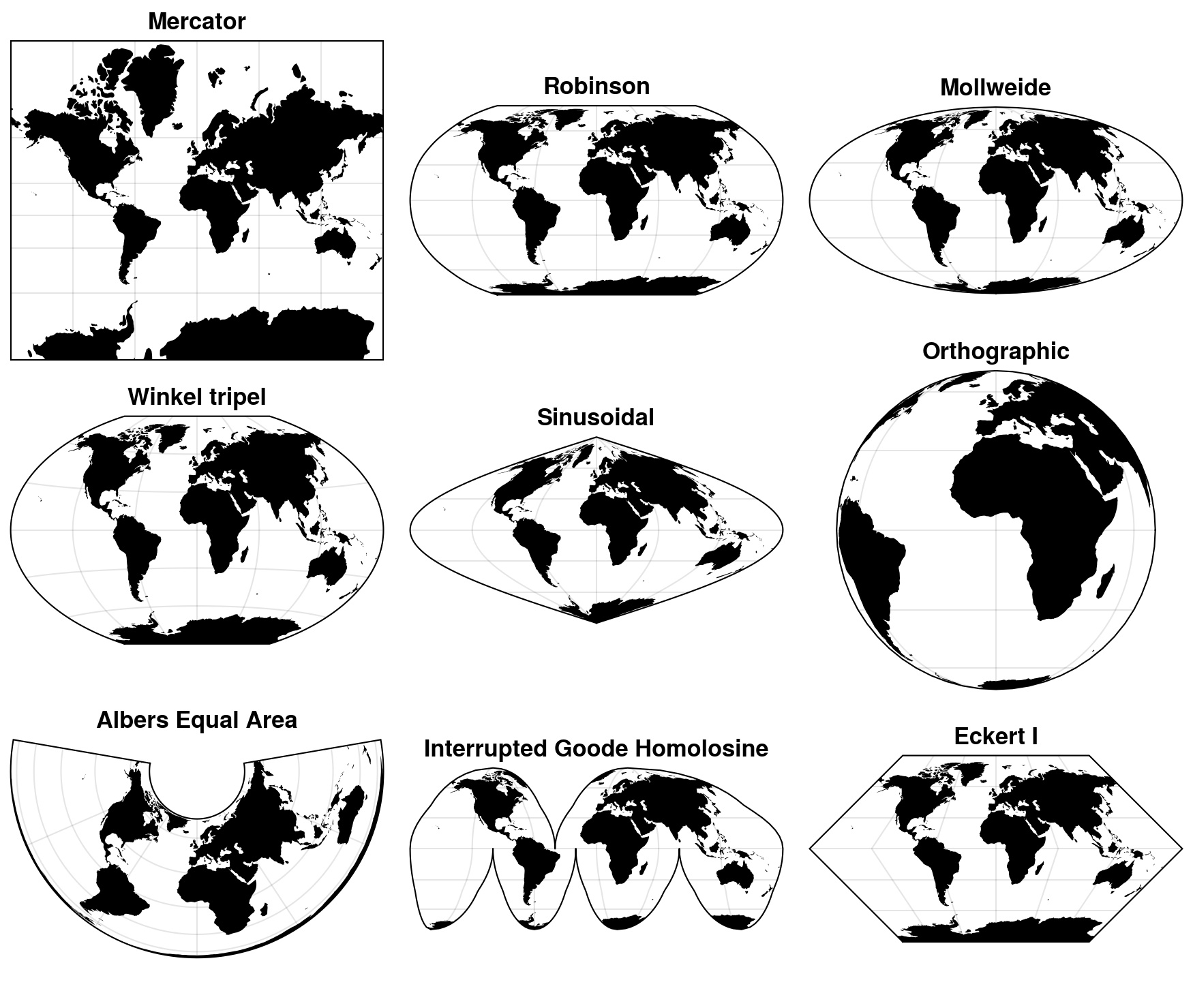
Because flattening the Earth requires compromise, cartographers have invented hundreds of different projections. Each one is designed for a specific purpose, prioritizing the preservation of shape, area, or distance. Source: Geopython
5. Exercise: The Flat Earth
Web Mercator (3857) is great for web navigation, but it notoriously distorts the size of objects near the poles (making Greenland look as big as Africa). For global scientific analysis, we prefer an “Equal Area” projection.
Your task is to reproject the world dataset into a flat, area-preserving projection and visually compare it to the original data.
Tasks:
Reproject: Create a new variable called
world_equal_area. Use.to_crs()on your originalworld_gdfto project it into the Equal Earth projection (EPSG:8857).Plot Original: Plot the original geographic dataset (
world_gdf) giving it a light grey color.Plot Projected: Plot your new
world_equal_areadataset right below it using a green color.Compare: Look closely at the visual difference between the two stacked maps, particularly the size of Greenland and Antarctica! Notice how the axis numbers have changed from degrees (e.g., -180 to 180) to millions of meters!
# Write your code here
Sample solution
# 1. Reproject to Equal Earth (EPSG:8857)
world_equal_area = world_gdf.to_crs(epsg=8857)

# 2. Plot the original Geographic CRS (Degrees)
world_gdf.plot(
    figsize=(10, 5),
    color="lightgrey",
    edgecolor="white"
);

# 3. Plot the new Projected CRS (Meters)
world_equal_area.plot(
    figsize=(10, 5),
    color="mediumseagreen",
    edgecolor="white"
);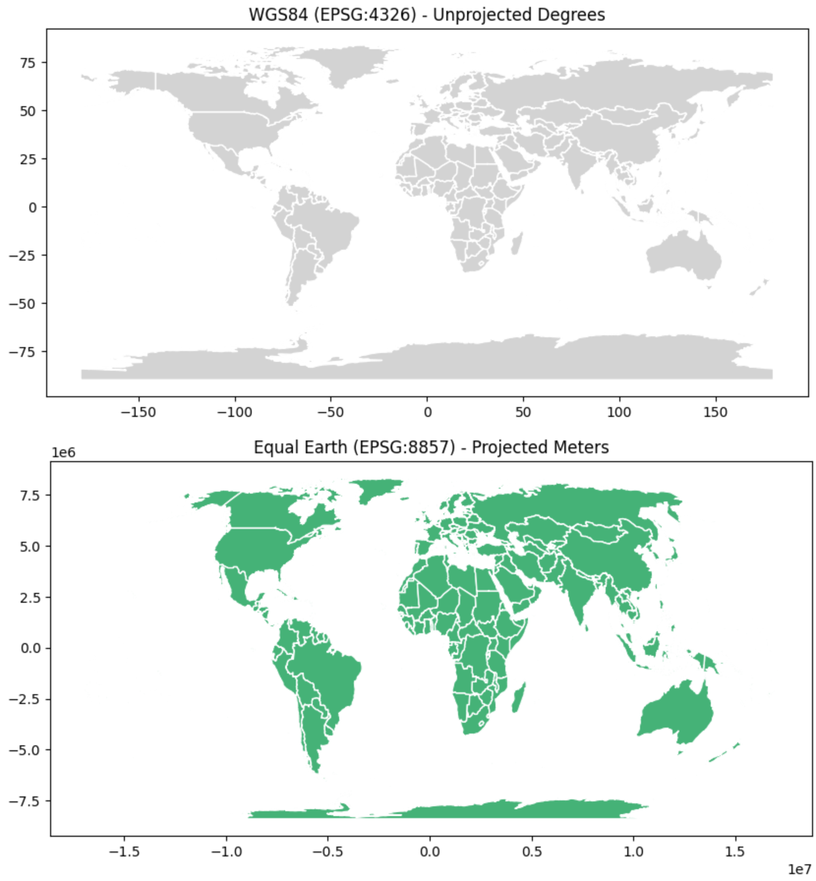
Stacked visual inspection of unprojected degrees (top) versus projected meters (bottom).
6. Summary: Managing Projections
In this section, you learned how to navigate the complexities of mapping a 3D Earth onto a 2D screen. Mastering these concepts will save you hours of debugging and prevent the vast majority of spatial errors you might encounter in the wild.
Key takeaways
The Two Families: Geographic coordinate systems use 3D degrees (ideal for global positioning), while Projected coordinate systems use 2D metric grids (essential for measuring areas and distances).
Checking Metadata: Always check
.crswhen loading new data. If the CRS is missing or incorrect, your spatial math will be wrong.EPSG Codes: Memorize the key shorthand codes. 4326 is your raw GPS data. 2056 is your highly accurate local Swiss grid.
The Master Tool: Use
.to_crs(epsg=XXXX)to effortlessly reproject your data. Always ensure two datasets are in the exact same CRS before trying to analyze them together!
What comes next?
Now that you know how to safely flatten the Earth onto a measurable metric grid, it is time to actually start measuring it.
Up to this point, we have only been loading and visualizing existing shapes. In the next section, Measuring and Modifying Geometries, we will move from simply holding spatial data to generating brand new geospatial metrics. You will learn how to calculate precise surface areas, find the exact center of a country, and draw proximity buffers around train stations to see exactly what falls inside their zone of influence!