Getting Data In and Out - Programming with Spatial Data

Learning to read and write data the easy way

One of the most useful features of pandas is its ability to interact with numerous data formats for both reading and writing. This includes common formats such as:

CSV and other delimited text files
JSON
HTML tables
Microsoft Excel files
SQL databases
HDF5, Stata, SAS, and Pickle

1. The Magic of read_csv()¶

Once you have acquired your data, the next step in every data science workflow is to load it. Pandas provides a single, highly optimised function for this: pd.read_csv().

We will load a dataset containing daily weather observations from the Kloten weather station in Zurich for the summer of 2022. You can download this dataset from: https://gitlab.com/HendrikWulf/sds210/-/blob/main/L06/data/kloten_summer_2022.txt and add it to your working directory on your local file system.

You might notice the file is named kloten_summer_2022.txt. Why use read_csv for a .txt file? File extensions are simply naming conventions. Whether a file ends in .csv, .txt, or .dat, if the internal contents are plain text separated by commas, pd.read_csv() is the correct tool to read it.

Let us look at the first 10 lines of the raw text file:

# Data file contents: Daily temperatures (TEMP1 (10:00), TEMP2 (14:00), MIN, MAX)
# for June 1 - August 31, 2022
# Data source: MeteoSwiss Open Government Data (OGD), station KLO
# Source URL (hourly data): [https://data.geo.admin.ch/ch.meteoschweiz](https://data.geo.admin.ch/ch.meteoschweiz)...
# Data processing: Extracted hourly air temperature...
# computed daily minimum and maximum temperatures...
# and 14:00 (TEMP2); formatted as comma separated values...
# Processed by Hendrik Wulf, 17.03.2026
YEARMODA,MAX,MIN,TEMP1,TEMP2
20220601,19.6,11.1,19.5,15.6

As we can see, the first 10 rows contain metadata comments starting with #. We do not want to load this text as data. Fortunately, skipping rows is easy using the skiprows parameter.

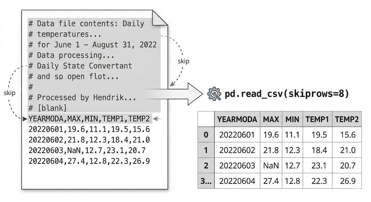
Conceptual diagram of the read_csv parsing process. — *The `read_csv` function automatically parses delimiters, detects headers, and assigns an index. Parameters like `skiprows` allow you to bypass messy metadata.*

import pandas as pd

# Read the data file, skipping the first 10 lines of metadata comments
data = pd.read_csv("kloten_summer_2022.txt", skiprows=10)

print("Data loaded successfully!")

(Note: Pandas has similar functions for other formats, such as pd.read_excel() for Excel files or pd.read_json() for JSON files.)

2. Quick Peeks (head and tail)¶

Data scientists rarely print entire datasets directly. Trying to display millions of rows will crash your browser window. Instead, we view small selections from the start or end of the data to verify it loaded correctly.

Pandas provides the .head() method, which returns the first five rows of a DataFrame by default. You can return any specific number of rows by placing an integer inside the parentheses.

# Check the first 4 rows
data.head(4)

Table 1:Output of data.head(4)

	YEARMODA	MAX	MIN	TEMP1	TEMP2
0	20220601	19.6	11.1	19.5	15.6
1	20220602	21.8	12.3	18.4	21.0
2	20220603	NaN	12.7	23.1	20.7
3	20220604	27.4	12.8	22.3	26.9

Notice that Pandas correctly identified our header row and automatically generated a sequential numeric Index on the far left. Also notice the NaN value in row 2. NaN stands for “Not a Number” and is how Pandas represents missing data.

Similarly, .tail() returns the last rows of the DataFrame.

# Check the last 3 rows
data.tail(3)

Table 2:Output of data.tail(3)

	YEARMODA	MAX	MIN	TEMP1	TEMP2
89	20220829	27.0	NaN	22.3	27.0
90	20220830	27.6	13.5	22.8	27.6
91	20220831	21.0	14.1	16.6	21.0

3. Exploring Metadata¶

After loading data, the standard “first 30 seconds” workflow is to explore the dataset’s metadata. This helps you understand the size and structure of your new object.

First, we check the dimensions using the .shape attribute. It returns a tuple representing (rows, columns).

data.shape

Output:

(92, 5)

Next, we extract the exact column names using .columns.values. This is incredibly helpful when working with datasets that contain hundreds of features, or to check if there are hidden spaces in the column names.

data.columns.values

Output:

array(['YEARMODA', 'MAX', 'MIN', 'TEMP1', 'TEMP2'], dtype=object)

Finally, the most powerful metadata tool is the .info() method. It provides a dense summary including row counts, missing values, and the data types (dtypes) of every column.

data.info()

<class 'pandas.core.frame.DataFrame'>
RangeIndex: 92 entries, 0 to 91
Data columns (total 5 columns):
 #   Column    Non-Null Count  Dtype  
---  ------    --------------  -----  
 0   YEARMODA  92 non-null     int64  
 1   MAX       82 non-null     float64
 2   MIN       87 non-null     float64
 3   TEMP1     92 non-null     float64
 4   TEMP2     92 non-null     float64
dtypes: float64(4), int64(1)
memory usage: 3.7 KB

This raw text block instantly tells us four critical pieces of information:

Total Rows: The second line (RangeIndex: 92 entries) confirms our dataset has exactly 92 rows.
Data Types: YEARMODA is stored as an integer (int64), while the temperatures are decimals (float64).
Missing Values: Because we know the total is 92 entries, we can see there are missing values in the MAX and MIN columns (which only have 82 and 87 non-null counts, respectively).
Memory Usage: The bottom line shows this tiny dataset is only using 3.7 KB of RAM. This check becomes vital later in your career when working with millions of rows!

Concept Check: Parentheses or not?¶

In the code above, why do we type data.info() with parentheses, but data.shape without them?

Check your understanding

.info() is a method (an action or tool the DataFrame executes, like calculating a summary). Methods always require parentheses to run.
.shape is an attribute (a static characteristic or property the DataFrame already knows about itself). Attributes do not use parentheses.

Think of it like a person: person.age is an attribute because it simply returns a stored fact (like the number 25). However, person.speak() is a method because it tells the person to actively perform an action (like saying “Hello!”).

4. Exporting Data (to_csv)¶

Once you finish cleaning, processing, or aggregating your data, you will want to save it back to your computer. Pandas uses the .to_csv() method for this task.

If you are working with other software, you can easily adapt this using methods like .to_excel() or .to_json().

The most critical parameter to remember when saving is index=False. If you omit this, Pandas will write the row labels (the 0, 1, 2 sequence) into the file as a brand new column. If you load that file again later, you will end up with an redundant column named Unnamed: 0.

# Define the output file name
output_file = "kloten_cleaned_summer_2022.csv"

# Save DataFrame to a new CSV file
# We use index=False to prevent saving the sequential row numbers
data.to_csv(output_file, index=False)

print("File successfully saved!")

5. Exercise: The Intake Workflow¶

To consolidate these steps, practice the standard intake workflow using a new dataset.

You can download a zip-file called simplemaps_worldcities_basicv1.901.zip using this link: https://simplemaps.com/static/data/world-cities/basic/simplemaps_worldcities_basicv1.901.zip. It contains a file called worldcities.csv, which you should extract and add to your working directory.

Tasks:

Load: Write the code to load the dataset into a variable named cities_df. (Assume there are no messy header comments this time).
Peek: Display the first 10 rows.
Shape & Columns: Print the shape of the DataFrame and an array of its column names.
Export: Save a copy of the data as worldcities_backup.csv, ensuring you do not save the index.

# Write your code here

Sample solution

import pandas as pd

# 1. Load
cities_df = pd.read_csv("worldcities.csv")

# 2. Peek
display(cities_df.head(10))

# 3. Shape & Columns
print(cities_df.shape)
print(cities_df.columns.values)

# 4. Export
cities_df.to_csv("worldcities_backup.csv", index=False)

6. Summary: File I/O and Inspection¶

In this section, we covered the essential data loading and saving pipeline. The goal of this phase is to make getting data in and out of your Python pipeline frictionless.

You learned how to:

Load Data: Use pd.read_csv() to parse text files (both .csv and .txt), leveraging parameters like skiprows to handle messy metadata headers.
Peek Safely: Use .head() and .tail() to inspect snippets of the data without crashing your environment.
Assess Metadata: Use .shape, .columns.values, and .info() to execute the critical “first 30 seconds” workflow to verify row counts, identify missing values, and check data types.
Export Cleanly: Save your data back to the hard drive using .to_csv(index=False), as well as understanding that tools like .to_excel() exist for other formats.

Now that the data is loaded and inspected, the next step is learning how to select specific rows and columns for analysis!