
In the previous section, we successfully loaded the kloten
import pandas as pd

# Load the Kloten summer weather data, skipping metadata
data = pd.read_csv("kloten_summer_2022.txt", skiprows=10)
1. Selecting Columns
When performing data analysis, you rarely need every variable in your dataset. You can extract specific columns by placing the column name inside square brackets next to your DataFrame variable.
To extract a single column, pass the name as a string. This returns a one dimensional Series.
# Extract a single column
max_temps = data["MAX"]

# Prove it is a Series
print(type(max_temps))

# Look at the first 3 rows
max_temps.head(3)
Output:
<class 'pandas.core.series.Series'>

0    19.6
1    21.8
2     NaN
Name: MAX, dtype: float64To extract multiple columns, you must pass a list of column names inside the square brackets. This means you will see double brackets [[ ]].
The outer brackets tell Pandas you are making a selection:
data[ ... ]The inner brackets define the Python list of strings:
["YEARMODA", "MAX", "MIN"]
Extracting multiple columns returns a smaller DataFrame, rather than a Series.
# Extract multiple columns
subset = data[["YEARMODA", "MAX", "MIN"]]

# Prove it is a DataFrame
print(type(subset))

display(subset.head(3))
Output:
<class 'pandas.core.frame.DataFrame'>Table 1:Output of multiple column selection
| YEARMODA | MAX | MIN | |
|---|---|---|---|
| 0 | 20220601 | 19.6 | 11.1 |
| 1 | 20220602 | 21.8 | 12.3 |
| 2 | 20220603 | NaN | 12.7 |
“Note: We use the display() function here to explicitly print the DataFrame as a cleanly formatted HTML table in our notebook.”
2. Filtering Rows
Selecting columns is easy, but how do we select specific rows? In pure Python, you would use an if statement to check each row one by one. In Pandas, we use a concept called Boolean Indexing to ask the entire dataset a True or False question simultaneously.
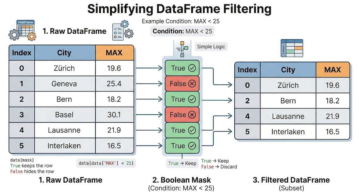
Boolean indexing conceptually acts as a filter. The mask of True/False values determines exactly which rows from the original DataFrame are allowed to pass through into your new subset.
First, we ask the question. Let us find out which days had a maximum temperature greater than 30 degrees Celsius:
# Ask the question (creates a boolean mask)
data["MAX"] > 30
Output:
0     False
1     False
2     False
3     False
      ...
88    False
89    False
90    False
91    False
Name: MAX, Length: 92, dtype: bool
This returns a Series of True and False values, often called a mask.
To actually filter the data, we place this conditional mask inside the selection brackets. Pandas will keep every row that evaluates to True and hide every row that evaluates to False.
For absolute clarity, here is how you do it in two steps:
# Step 1: Save the mask to a variable
is_hot = data["MAX"] > 30

# Step 2: Pass the mask variable into the brackets
hot_days = data[is_hot]
However, experienced programmers usually combine this into a single line of code by placing the condition directly inside the brackets. Notice how the word data appears twice:
# The standard one-line approach
hot_days = data[data["MAX"] > 30]

display(hot_days.head(3))
Table 2:Output of hot_days
| YEARMODA | MAX | MIN | TEMP1 | TEMP2 | |
|---|---|---|---|---|---|
| 15 | 20220616 | 30.1 | 17.0 | 27.3 | 29.9 |
| 18 | 20220619 | 35.1 | 17.1 | 30.0 | 34.8 |
| 19 | 20220620 | 30.9 | 18.9 | 27.4 | 30.7 |
Notice the Index on the far left. It jumped from 15 to 18 to 19, preserving the original row labels of the days that met our criteria.
3. Multiple Conditions
Often, you need to filter data using multiple criteria simultaneously. You can combine logical conditions using special operators. Standard Python keywords and and or will not work here, as Pandas needs bitwise operators that perform vectorized logical comparisons on entire Series at once.
Pandas uses these operators:
&(AND): Both conditions must be True.|(OR): At least one condition must be True.
AND Condition Example
Let us find “extreme” summer days that were both very hot (MAX > 30) but also had surprisingly cool mornings (MIN < 14).
# Using & (AND) for logical conditions
extreme_days = data[(data["MAX"] > 30) & (data["MIN"] < 14)]
display(extreme_days)
Table 3:Output of hot days with cool mornings
| YEARMODA | MAX | MIN | TEMP1 | TEMP2 | |
|---|---|---|---|---|---|
| 32 | 20220703 | 30.1 | 13.5 | 25.7 | 29.8 |
| 47 | 20220718 | 32.4 | 13.0 | 27.6 | 32.0 |
OR Condition Example
Next, let us find days that were either extremely hot (MAX > 33) OR had very cold mornings (MIN < 10). This query will include days meeting either criteria, or both.
# Using | (OR) logic for extreme temperatures
either_extreme_days = data[(data["MAX"] > 33) | (data["MIN"] < 10)]
display(either_extreme_days)
Table 4:Output of days with either extreme MAX or MIN
| YEARMODA | MAX | MIN | TEMP1 | TEMP2 | |
|---|---|---|---|---|---|
| 10 | 20220611 | 25.6 | 9.1 | 21.8 | 25.1 |
| 13 | 20220614 | 25.9 | 9.9 | 21.6 | 25.8 |
| 18 | 20220619 | 35.1 | 17.1 | 30.0 | 34.8 |
| 49 | 20220720 | 33.4 | 17.5 | 30.4 | 32.9 |
| 51 | 20220722 | 33.4 | 14.1 | 26.5 | 31.5 |
| 54 | 20220725 | 34.2 | 16.4 | 30.4 | 34.2 |
| 65 | 20220805 | 33.4 | 19.1 | 29.5 | 33.0 |
4. Sorting Data (sort_values)
Once you have isolated your data, you frequently want to order it. The .sort_values() method allows you to sort your DataFrame by one or more columns.
By default, Pandas sorts in ascending order (smallest to largest). To find the absolute hottest days of the summer at the top of our table, we need to set the ascending parameter to False.
# Sort by MAX temperature, descending
sorted_data = data.sort_values(by="MAX", ascending=False)
display(sorted_data.head(3))
Table 5:Output of sorted_data
| YEARMODA | MAX | MIN | TEMP1 | TEMP2 | |
|---|---|---|---|---|---|
| 18 | 20220619 | 35.1 | 17.1 | 30.0 | 34.8 |
| 54 | 20220725 | 34.2 | 16.4 | 30.4 | 34.2 |
| 64 | 20220804 | 33.7 | 15.1 | 27.7 | 32.6 |
5. The View vs Copy Trap
When you filter a DataFrame (like we did with hot_days), Pandas tries to be as efficient as possible with your computer’s memory. Instead of automatically creating a brand new data object, it often returns a view.
Because a view is still linked to the original DataFrame, changing the data inside the view can accidentally alter your original dataset! To prevent you from doing this, Pandas monitors your code. If you try to modify a view, it will throw a massive warning block called a SettingWithCopyWarning.
Let us look at how this happens. Suppose we filter our data for early June and try to add a new column to it:
# 1. We create a subset (this creates a view, not a copy!)
early_june = data[data["YEARMODA"] < 20220610]

# 2. We try to modify this subset by adding a new column
early_june["IS_HOT"] = early_june["MAX"] > 25
Output:
SettingWithCopyWarning:
A value is trying to be set on a copy of a slice from a DataFrame.
Try using .loc[row_indexer,col_indexer] = value instead

See the caveats in the documentation: [https://pandas.pydata.org/pandas-docs/stable/user_guide/indexing.html#returning-a-view-versus-a-copy](https://pandas.pydata.org/pandas-docs/stable/user_guide/indexing.html#returning-a-view-versus-a-copy)
Pandas is warning you: “Hey, you are trying to change a slice of data that is still linked to the original DataFrame. This could cause unpredictable bugs!”
Proving the Linkage
To truly understand the danger, let us demonstrate what happens when data objects remain linked.
# Extract just the MAX temperatures (this is a view)
max_temps_view = data["MAX"]

# Let's maliciously change the FIRST value in the ORIGINAL dataset
data.iloc[0, 1] = 99.9

# Let's check our view...
print(f"New first value in view: {max_temps_view.iloc[0]}")
Output:
New first value in view: 99.9Even though we never touched max_temps_view directly, its value changed because it is permanently linked to the data DataFrame!
The Solution: Use .copy()
To avoid this trap entirely, always use the .copy() method at the end of your filtering statement if you plan to modify the subset later.
# Safe: We append .copy() to create an independent dataset
early_june_safe = data[data["YEARMODA"] < 20220610].copy()

# Now we can modify it without warnings or hidden linkages!
early_june_safe["IS_HOT"] = early_june_safe["MAX"] > 25
print("Column successfully added to the independent copy.")
Concept Check: To copy or not to copy?
Imagine you are writing a script to analyze weather patterns.
Scenario A: You filter the dataset to find all days where the minimum temperature dropped below 0°C, just so you can print them to the screen and read them. Scenario B: You filter the dataset to find all days with missing temperature readings, because you plan to overwrite those missing values with an average temperature.
In which scenario is it absolutely critical to use .copy()?
Check your understanding
Scenario B requires .copy().
In Scenario A, you are only reading the data (printing it to the screen). It is perfectly fine (and memory efficient!) to use a view for reading.
In Scenario B, you plan to modify the subset (overwriting missing values). If you don’t use .copy(), you will trigger a SettingWithCopyWarning, and you risk accidentally altering the original dataset in unpredictable ways. Rule of thumb: If you plan to alter the subset, always copy!
6. Index based Selection (loc vs iloc)
Up until now, we have selected columns by their names and rows by conditions. But what if you just want to grab the 5th row, regardless of what data is inside it? Pandas offers two specific tools for this:
.loc[](Label-based): Selects data based on its exact label (the name of the index row or the name of the column)..iloc[](Integer position-based): Selects data based on its strict numerical position (0, 1, 2...), exactly like a standard Python list.
![A conceptual diagram showing a Pandas DataFrame with a sorted, non-sequential index. An arrow for .loc[0] points to the specific row labeled '0', while an arrow for .iloc[0] points to the physical top row of the table.](/sds210-jb/build/06_loc_vs_iloc_index-7e858051ca0c7276a8f50fb40882f929.png)
Understanding the difference between label-based (.loc) and position-based (.iloc) indexing. When data is sorted, the physical position (0) no longer matches the original row label (0).
Let us look at the difference. Imagine we sort our data so the hottest day (originally Index 18) is at the very top of the table.
# 1. .iloc looks for the row currently sitting in the very first position (position 0)
print("Result of .iloc[0]:")
print(sorted_data.iloc[0])

print("\n-------------------\n")

# 2. .loc looks for the row literally labeled '0' (which is now deep in the middle of the sorted data)
print("Result of .loc[0]:")
print(sorted_data.loc[0])
Output:
Result of .iloc[0]:
YEARMODA    20220619.0
MAX               35.1
MIN               17.1
TEMP1             30.0
TEMP2             34.8
Name: 18, dtype: float64

-------------------

Result of .loc[0]:
YEARMODA    20220601.0
MAX               19.6
MIN               11.1
TEMP1             19.5
TEMP2             15.6
Name: 0, dtype: float64
Notice how .iloc[0] returned the data for the hottest day (labeled 18), while .loc[0] hunted down the specific row labeled 0 (June 1st).
Selecting Rows AND Columns
The true power of these indexers is that you can select rows and columns at the same time by separating them with a comma: [rows, columns].
# Use .loc to get rows labeled 0 through 3, and specifically the "MAX" and "MIN" columns
subset_loc = data.loc[0:3, ["MAX", "MIN"]]
display(subset_loc)
Output of .loc[0:3, [“MAX”, “MIN”]]
| MAX | MIN | |
|---|---|---|
| 0 | 19.6 | 11.1 |
| 1 | 21.8 | 12.3 |
| 2 | NaN | 12.7 |
| 3 | 27.4 | 12.8 |
7. Exercise: Isolate the Target Data
Let us bring all these skills together using the global cities dataset you downloaded in the previous section.
Imagine you are doing an analysis focused solely on major urban centers in Japan. You need to load the data, extract exactly what you need, and secure it in memory.
Tasks:
Load
worldcities.csvinto a DataFrame.Filter the data to include only rows where the
countrycolumn is exactly"Japan".Crucial: Make sure to append
.copy()to create an independent dataset!Sort this new Japan DataFrame by the
populationcolumn in descending order (largest to smallest).Display the top 5 rows, but only show the
cityandpopulationcolumns.
(Hint for Step 5: Remember that selecting multiple columns requires a list inside the selection brackets, which looks like double brackets [[ ]]).
# Write your code here
Sample solution
import pandas as pd

# 1. Load the data
cities_df = pd.read_csv("worldcities.csv")

# 2 & 3. Filter for Japan AND create a safe copy
japan_cities = cities_df[cities_df["country"] == "Japan"].copy()

# 4. Sort by population descending
japan_sorted = japan_cities.sort_values(by="population", ascending=False)

# 5. Extract specific columns and show the top 5
top_japan_cities = japan_sorted[["city", "population"]]
display(top_japan_cities.head(5))
Expected Output:
| city | population | |
|---|---|---|
| 0 | Tokyo | 37785000.0 |
| 23 | Ōsaka | 15126000.0 |
| 45 | Nagoya | 9197000.0 |
| 197 | Yokohama | 3757630.0 |
| 366 | Fukuoka | 2286000.0 |
(Note: The exact index numbers on the left might differ slightly depending on the version of the dataset, but the top 5 cities and populations should match!)
8. Summary: Navigating the 2D Grid
In this section, you learned how to slice and dice your data to extract exactly the information you need. You now have the tools to surgically navigate large datasets without relying on manual for loops.
Key takeaways
Columns: Extract a single Series using
df["col"]or a smaller DataFrame using a listdf[["col1", "col2"]].Rows: Use Boolean Indexing (
df[df["col"] == value]) to act as a filter, keeping only rows that meet logical conditions.Conditions: Combine multiple filters using
&(AND) or|(OR), always wrapping each individual condition in parentheses().Sorting: Use
.sort_values(by="col", ascending=False)to order your DataFrame.Safety: Always append
.copy()when filtering a DataFrame if you intend to modify the resulting subset later to avoid theSettingWithCopyWarning.Index Selection: Use
.iloc[]to select rows based on their strict numerical position, and.loc[]to select based on exact row/column labels.
What comes next?
Now that you can navigate, slice, and filter your data, you might notice a glaring issue: real-world data is rarely perfect.
If you try to do math on a column where numbers are accidentally stored as text, or if a sensor went offline and left blank gaps in your dataset, your code will crash. In the next section, Cleaning the Mess, we will learn how to standardize messy column headers, fix text strings, and handle the infamous NaN (Not a Number) so your data is pristine and ready for analysis!