
In the previous sections, you learned how to write your own custom modules and how to unlock the tools bundled in the Python Standard Library. This gave you a solid foundation. However, Python truly shines because of its massive open source ecosystem.
When you want to perform specialized tasks like processing geospatial polygons, creating interactive maps, or visually tracking your code’s progress, the Standard Library is not quite enough. This is where third party modules come in.
1. The open source ecosystem
A third-party module (often called a package or library) is simply a collection of code written by other programmers and made available for the public to use. There are hundreds of thousands of these packages available, covering almost any problem you can imagine.
Because they are created by the community and not the core Python team, they do not come preinstalled on your computer. You must actively download them before you can use them in your scripts or notebooks.
2. Package managers
To get these external tools onto your computer, we use package managers. You can think of a package manager as an app store for code. It finds the software you request, downloads it, and figures out if it needs any other supporting software (dependencies) to run properly.
As discussed in the environment setup chapter, there are two main package managers you will encounter:
pip: The default Python package installer. It downloads packages from the Python Package Index (PyPI).
conda: A powerful manager that handles Python packages as well as complex system software (like C++ libraries). This makes it the preferred choice for geospatial data science, where tools often rely on heavy external libraries.
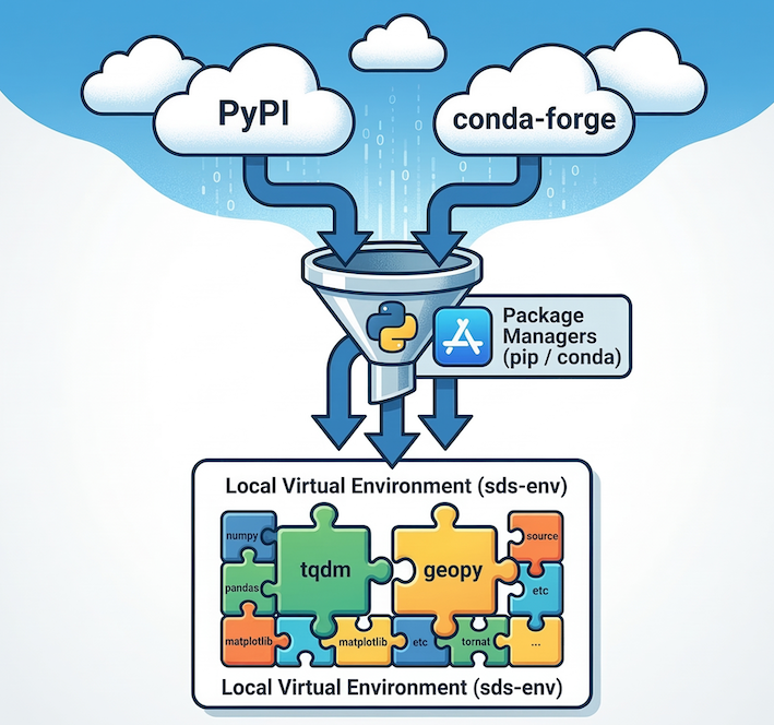
Package managers act as an app store for code, fetching external libraries from cloud repositories (like PyPI or conda-forge) and installing them safely into your local virtual environment.
3. Installing external packages
You cannot install a package from inside a standard Python script. Installation happens in your command line interface (like Anaconda Prompt or your system Terminal).
To keep your projects stable, you should always ensure your project specific virtual environment is active before installing new tools.
If you wanted to install a package for progress bars and a package for geospatial calculations, you would run commands like this in your terminal (using the conda-forge community channel):
# Ensure your environment is active first
conda activate sds-env

# Install packages using conda
conda install -c conda-forge tqdm geopy
Once a package is installed in your active environment, it stays there. You only need to install it once per environment.
4. Importing and exploring
Once a third party package is installed, bringing it into your notebook is exactly the same as importing your own scripts or the Standard Library.
from tqdm import tqdm
import geopy
Because third party libraries can be massive, the dir() and help() functions you learned about earlier might output an overwhelming amount of information. For community packages, your best approach is to read the official online documentation. Most popular packages host comprehensive guides and tutorials on websites like Read the Docs.
5. Practical example: Tracking progress
Let us look at a highly popular third-party module called tqdm (which comes from the Arabic word taqaddum, meaning “progress”).
In the previous chapter, you learned how to write for loops. When a loop processes a massive dataset, it can take minutes or hours to finish, and by default, Python will not tell you how far along it is. The community built tqdm to instantly add a smart progress bar to any loop.
To demonstrate how this works, we will also use the time module. Unlike tqdm, which is a third-party package you must install, time is built directly into Python’s standard library, so it is always available right out of the box.
import time
from tqdm import tqdm

# We wrap our range() with tqdm() to automatically generate a progress bar
for i in tqdm(range(5)):
    # Simulate a task that takes 0.5 seconds to complete
    time.sleep(0.5)
Understanding the code
import time: This brings in Python’s built-in time tools. We usetime.sleep(0.5)to artificially pause the loop for half a second, simulating a task that takes time to compute.from tqdm import tqdm: This syntax might look like a typo, but there is a specific reason it’s written twice! The firsttqdmis the name of the library itself (the folder of code you installed). The secondtqdmis the specific function (technically a class) inside that library that actually draws the progress bar.
By simply wrapping our sequence in tqdm(), we get a visual progress bar, a percentage completed, and an estimated time remaining, all in a single line of code.
Concept check
Look closely at our import statement:
from tqdm import tqdm
If we changed our code to instead read:
import tqdm
How would you have to rewrite the loop initialization line (for i in tqdm(range(5)):) to make it work without crashing?
Test your namespace knowledge!
You would have to write:
for i in tqdm.tqdm(range(5)):
Why?
When you write import tqdm, you are importing the entire module (the folder of code) named tqdm. To use the specific progress-bar function (which is also named tqdm) inside that folder, you must use dot notation: module.function(), which results in tqdm.tqdm().
Using from tqdm import tqdm skips the folder name and pulls the specific function directly into your main workspace, allowing you to just write tqdm().
6. Practical example: Spatial distance
In the previous sections, you wrote your own function for Euclidean distance and used the math module to calculate Haversine distance.
Writing complex math formulas yourself is prone to typos. Instead, we can trust the geopy package, which has been rigorously tested by thousands of developers.
This function calculates the shortest geodesic distance between two points on the surface of the Earth. Instead of treating the Earth as a perfect sphere, geopy uses a highly accurate ellipsoidal model (WGS-84) by default. It accepts coordinates in (latitude, longitude) order, and can output the distance in kilometers, meters, or miles.
from geopy import distance

# Define our coordinates (lat, lon) as tuples
kolkata = (22.5246, 88.3432)
hanoi = (21.0291, 105.8358)

# Use geopy to calculate the highly accurate geodesic distance
true_distance = distance.geodesic(kolkata, hanoi).km

print(f"Distance: {true_distance:.1f} km")
By leveraging third party code, we replaced a complicated math function with a single, highly readable line of code.
7. Best practices
When working with external code, keep these professional habits in mind:
Document your dependencies: Because your code now relies on external tools, anyone else who wants to run your notebook needs to install those same tools. Always keep a list of the packages you use (often saved as an
environment.ymlorrequirements.txtfile).Read the docs: Before you write a complex function, do a quick web search. Chances are, a third party package already exists that does exactly what you need.
Check the license: Open source code is free, but different packages have different rules about how they can be used, especially in commercial projects.
8. Exercises
Practice managing and using third party modules with these tasks.
Exercise 1: Planning an e-motorcycle tour
The tqdm library makes tracking long tasks incredibly easy. Let us use it to plan an epic e-motorcycle tour down the Andes mountains in South America, calculating the distance of each leg of the trip.
We have provided a list of cities in geographical order from north to south, along with their coordinates.
Import
tqdmfrom thetqdmmodule,timefrom the Standard Library, anddistancefromgeopy.Create a variable called
total_distanceand set it to0.Write a
forloop to iterate through the list. Since we need to measure the distance between the current city and the next city, loop overrange(len(route) - 1)and wrap this range intqdm().Inside the loop, extract the coordinates for the current city and the next city.
Calculate the geodesic distance between them in kilometers and add it to
total_distance.Use
time.sleep(1)to pause for one second so you can watch the progress bar update.Print the final cumulative distance after the loop finishes.
# Copy this list into your script
route = [
    ("Bogotá", (4.7110, -74.0721)),
    ("Quito", (-0.1807, -78.4678)),
    ("Lima", (-12.0464, -77.0428)),
    ("La Paz", (-16.4897, -68.1193)),
]
Sample solution
import time
from tqdm import tqdm
from geopy import distance

# Our Andean motorcycle route
route = [
    ("Bogotá", (4.7110, -74.0721)),
    ("Quito", (-0.1807, -78.4678)),
    ("Lima", (-12.0464, -77.0428)),
    ("La Paz", (-16.4897, -68.1193))
]

total_distance = 0

print("Calculating tour distances...")

# We loop through the route indices, stopping before the last city
for i in tqdm(range(len(route) - 1)):

    # Get the coordinates for the current and next city
    current_city, current_coords = route[i]
    next_city, next_coords = route[i + 1]

    # Calculate the distance of this specific leg
    leg_distance = distance.geodesic(current_coords, next_coords).km
    total_distance += leg_distance

    # Pause to simulate heavy processing and watch the progress bar!
    time.sleep(1)

print(f"\nTotal tour distance: {total_distance:.1f} km")
Key idea:
Third-party modules abstract away the hard parts. tqdm handles all the complex time calculations and visual formatting behind the scenes, while geopy handles the intense spatial math, leaving you free to focus on the logic of planning your trip!
Exercise 2: Measuring the Earth’s bulge
The Earth is not a perfect sphere. Because of its rotation, it bulges outward at the equator and is slightly flattened at the poles.
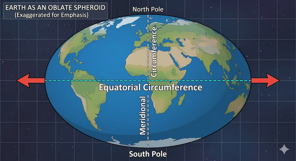
Due to its rotation, the Earth is not a perfect sphere but an oblate spheroid, bulging at the equator and slightly flattened at the poles.
Use the geopy package to calculate the exact difference. Because geopy uses the WGS-84 ellipsoid model of the Earth by default, it perfectly accounts for this equatorial bulge.
Import
distancefromgeopy.To measure the equator, create points at
(0, 0)and(0, 90).To measure the meridian, create points at
(0, 0)and the North Pole(90, 0).Calculate the geodesic distance for both quarter-circles in kilometers.
Multiply both by 4 to estimate the full circumferences, then print their difference.
# Write your code here
Sample solution
from geopy import distance

# Equator points (moving along the equator)
eq_point1 = (0, 0)
eq_point2 = (0, 90)

# Meridian points (moving from equator to North Pole)
mer_point1 = (0, 0)
mer_point2 = (90, 0)

# Calculate a quarter of the Earth for both
quarter_equator = distance.geodesic(eq_point1, eq_point2).km
quarter_meridian = distance.geodesic(mer_point1, mer_point2).km

# Estimate full circumferences
circ_equator = quarter_equator * 4
circ_meridian = quarter_meridian * 4

difference = circ_equator - circ_meridian

print(f"Equator Circumference: {circ_equator:.1f} km")
print(f"Meridian Circumference: {circ_meridian:.1f} km")
print(f"The equator is {difference:.1f} km longer!")
Key idea:
If you guessed B (~67 km), you were right! You can trust established community packages to handle complex geometries like the WGS-84 ellipsoid under the hood. Writing the complex math to calculate distances on an oblate spheroid by hand would be incredibly tedious, but geopy handles it in a single line.
9. Summary
In this section, you learned how to break out of the built in Python ecosystem and utilize the vast library of community tools. You discovered how to:
Identify the difference between the Standard Library and third party modules.
Understand the role of package managers like
condaandpip.Import and use external libraries just like your own local scripts.
Use
tqdmto instantly add visual progress bars to your loops.Use
geopyto calculate highly accurate spatial distances.
What comes next?
You now know how to extend Python with powerful community tools. But what if the data you need isn’t saved on your computer?
In the next section, Using Web APIs, you will learn how to connect Python directly to the live internet. You will discover how to use the requests module to ask remote servers for exact data—like live weather forecasts and historical climate records—and pull it straight into your code without ever opening a web browser.