
Now that you understand why functions matter, it is time to look under the hood. In this section, we will build functions from scratch. We will start with a simple spatial calculation, explore how to pass geographic data into our tools safely, and clear up one of the most common beginner misunderstandings: the difference between printing a value and returning one.
1. The Anatomy of a Function
Every function in Python has a specific, predictable structure. A function is defined using the def keyword.
Here is the blueprint:
def function_name(parameters):
    # The body of the function (indented)
    return value
Let’s break down the components:
def: Short for “define.” This keyword tells Python you are creating a new function.Name: A good function name is verb-based because functions do things (e.g.,
calculate_distance,clean_data).Parameters: The variable names inside the parentheses. You can pass data as parameters into a function that are used as arguments. Think of these as empty, labeled mailboxes waiting for a data delivery (inputs).
return: The keyword that sends the final output back to the main program so it can be saved, modified, or used later.
First Example: Calculating a Buffer Area
Let’s translate a formal mathematical formula into a Python function. In spatial analysis, you may want to calculate the area of a circular “buffer” around a specific coordinate (for example, a 50-meter protection zone around a nesting site).
The formula for the area of a circle is: .
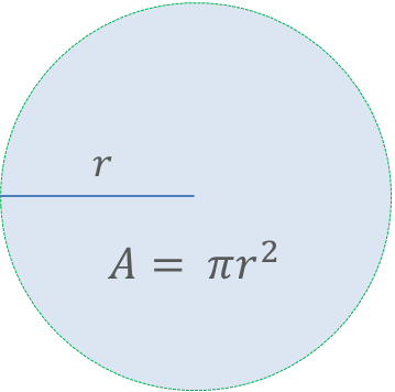
Calculating the area of a circular buffer zone using its radius ().
Here is how we package that logic into a function:
def calculate_buffer_area(radius):
    return 3.14159 * (radius**2)
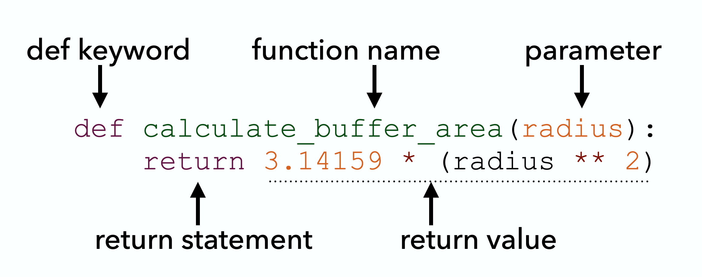
This is an example function, annotated to highlight its important elements.
To use it, we simply call the function by its name and pass it a number. We can then store the result in a variable or embed it directly into a print() statement:
# Calling the function and storing the result
nesting_zone_area = calculate_buffer_area(50)

# Embedding the function call inside an f-string
print(f"A 100 m buffer covers {calculate_buffer_area(100)} square meters.")
2. Parameters and Arguments
Wait, aren’t parameters and arguments the exact same thing? This is a very common stumbling block! They are closely related, but they play distinct roles depending on whether you are building the tool or using the tool:
Parameter: The placeholder name used when defining the function (e.g.,
radius). Think of it as an empty, labeled mailbox waiting for a delivery.Argument: The actual data value passed into the function when you call it (e.g.,
50). This is the actual package you drop into that mailbox.
When you pass data into a function, Python needs a set of rules to figure out which argument belongs to which parameter. There are two main ways to do this:
1. Positional Arguments
By default, Python assigns arguments to parameters based strictly on their order.
Let’s look at our previous buffer area example. If we define calculate_buffer_area(radius), calling calculate_buffer_area(50) maps the value 50 directly to the radius parameter because it is first in line.
2. Keyword Arguments
Instead of relying on order, you can explicitly state the parameter name in the function call. When you use keyword arguments, the order no longer matters.
# Calling the function using a keyword argument
calculate_buffer_area(radius=50)
Why Keyword Arguments Matter in Spatial Data
In simple functions with one input, positional arguments are perfectly fine. But geospatial programming often requires passing multiple coordinates at once.
Imagine calculating the distance between two points on Earth using their latitudes and longitudes. Because the Earth is spherical, we cannot use a simple straight line; we must use the Haversine formula to calculate the great-circle distance.

A diagram illustrating great-circle distance (drawn in red) between two points on a sphere.
Here is what that function looks like in Python:
from math import radians, sin, cos, sqrt, atan2


def haversine(lat1, lon1, lat2, lon2):
    R = 6371.0  # Earth radius in kilometers
    dlat = radians(lat2 - lat1)
    dlon = radians(lon2 - lon1)

    a = (
        sin(dlat / 2) ** 2
        + cos(radians(lat1)) * cos(radians(lat2)) * sin(dlon / 2) ** 2
    )
    c = 2 * atan2(sqrt(a), sqrt(1 - a))

    distance = R * c
    return distance
Look at the four parameters required by this function: lat1, lon1, lat2, lon2. If you use positional arguments, your function call looks like a random string of numbers.
For example, let’s calculate the distance between Beirut (33.8869° N, 35.5131° E) and Jerusalem (31.7683° N, 35.2137° E). Because the latitudes and longitudes are numerically very similar, positional arguments can become a trap:
# BAD: All these numbers look similar (31-35). Did I pass Lat/Lon or Lon/Lat?
dist = haversine(33.8869, 35.5131, 31.7683, 35.2137)
This is incredibly dangerous in spatial analysis. If you accidentally provide the longitude first (35.5131, 33.8869), Python won’t throw an error. It will just quietly place your data point 200 kilometers away, floating in the middle of the Mediterranean Sea!
Using keyword arguments makes your code self-documenting, safe, and highly readable:
# GOOD: Clear, safe, and readable.
dist = haversine(lat1=33.8869, lon1=35.5131, lat2=31.7683, lon2=35.2137)

# Because we used keywords, we can even safely change the order!
# (Many spatial systems use X/Y or Lon/Lat ordering, so this is very useful)
dist = haversine(lon1=35.5131, lat1=33.8869, lon2=35.2137, lat2=31.7683)
3. Return Values vs Printing
If there is one concept to master in this section, it is this: Printing is not Returning. This is a key concept in programming. Once you grasp it, the way you write and connect code will change noticeably.
Here is the core difference:
print()is for humans. It displays text on your screen so you can read it, but the computer immediately forgets that data.returnis for the computer. It hands the data back to the program’s memory so it can be stored in a variable, modified, or passed into another function.
Let’s look at the difference in action by creating two functions that calculate population density, but handle the output very differently:
# Function 1: Only prints the result to the screen
def print_density(population, area):
    print(population / area)


# Function 2: Returns the result to the computer's memory
def calculate_density(population, area):
    return population / area
If you just run print_density(5000, 10), the number 500.0 appears on your screen. It looks like it worked perfectly! But what happens if we try to capture that output and save it to a variable for our spatial analysis?
output = print_density(5000, 10)
print("The stored output is:", output)
Output:
500.0
The stored output is: None
The None Trap
Why did the second print statement say None?
Because print_density never officially handed any data back using a return statement. It just flashed the number on the screen and vanished. Functions with no return statement will automatically return None. None is Python’s way of representing “nothing”.
If you try to do math with None later in your code, your program will crash.
The Solution: Always Return
If you want to use the result of a function later in your code, you must use return.
# This works! The data is saved in memory.
output = calculate_density(5000, 10)
print("The stored output is:", output)
Output:
The stored output is: 500.0
4. Functions Calling Functions
Now that we know functions must return data to the computer’s memory, we can unlock the true power of programming: composition.
Because a return statement hands data back to the program, the output of one function can be fed directly into the input of another. Instead of writing one massive, complex function that tries to do ten different things, professional programmers write ten small, simple functions that each do one thing perfectly. Then, they snap them together like building blocks.
Let’s look at how this works. Suppose we know the radius of a city limit in kilometers, as well as its total population, and we want to find the population density.
We already built a tool to calculate density. Let’s build a quick tool to calculate the area based on the radius:
# Tool 1: Calculate Area
def calculate_area(radius):
    return 3.14159 * (radius**2)


# Tool 2: Calculate Density
def calculate_density(population, area):
    return population / area
Now, we can simply build a new function that calls the tools we already made!
# Tool 3: Combining our existing tools
def estimate_city_density(population, radius):
    # Step 1: Call the first function and save its returned data
    city_area = calculate_area(radius)

    # Step 2: Pass that saved data into the second function, and return the final result
    return calculate_density(population, city_area)


# Testing our modular function
density = estimate_city_density(50000, 5)
print(f"The estimated density is {density} people per square kilometer.")
Thinking Like a Software Designer
Why is this approach so powerful for spatial data science?
Imagine you are processing messy GPS coordinates. You might build one function to clean the text (clean_coordinates), another to convert the format (dms_to_decimal), and a third to calculate the distance (haversine).
By keeping these functions separate and letting them call each other, your code becomes modular. If you realize you made a mistake in your text-cleaning logic, you only have to fix the clean_coordinates function. Because your other tools just call that function, fixing it in one place automatically fixes your entire pipeline.
This is the essence of good software design: solve a small problem once, and reuse that solution everywhere.
5. Exercises: Tracking the Great Migration
To truly master functions, we need a realistic scenario. In spatial ecology, tracking bird migrations and modeling habitat connectivity is a massive computational task. We have collected raw GPS data from 10 major wildlife bird reserves scattered across all four hemispheres (NE, SE, SW, NW).

Examples of long-distance bird migration routes. Source: Wikipedia
Many migratory birds are capable of staggering non-stop flights spanning thousands of kilometers. To understand their global networks, ecologists must calculate the exact distances between resting sites to determine which reserves fall within a species’ maximum flight range.
Here is our raw data in Degrees, Minutes, and Seconds (DMS):
reserves = {
    # North-West (Americas)
    "Yukon Delta, USA": {"lat": "61 00 00.0", "lon": "-163 00 00.0"},
    "Bear River, USA": {"lat": "41 27 00.0", "lon": "-112 17 00.0"},
    # South-West (Americas)
    "Paracas, Peru": {"lat": "-14 15 00.0", "lon": "-76 14 00.0"},
    "Tierra del Fuego, ARG": {"lat": "-54 50 00.0", "lon": "-68 28 00.0"},
    # North-East (Eurasia)
    "Wadden Sea, NLD": {"lat": "53 15 00.0", "lon": "5 15 00.0"},
    "Kushiro, JPN": {"lat": "43 06 00.0", "lon": "144 19 00.0"},
    "Keoladeo, IND": {"lat": "27 10 00.0", "lon": "77 31 00.0"},
    # South-East (Africa/Australasia)
    "Kakadu, AUS": {"lat": "-13 02 00.0", "lon": "132 26 00.0"},
    "Kruger, ZAF": {"lat": "-23 50 00.0", "lon": "31 30 00.0"},
    "Fiordland, NZL": {"lat": "-45 25 00.0", "lon": "167 43 00.0"},
}
Let’s build a modular toolkit to find out which reserves are connected on valid migratory routes!
Exercise 1: Cleaning the Coordinates (Core)
Before we can calculate flight paths, we must clean our data. GPS devices often output coordinates as strings in Degrees, Minutes, and Seconds (DMS), but spatial analysis in Python requires numeric Decimal Degrees (DD).
To calculate decimal degrees, we can use the formula below:
If degrees are positive:
If degrees are negative:
Your Task: Write a function called dms_string_to_decimal(dms_string) that takes a single coordinate string formatted with spaces.
Use the string
.split()method to break the string into a list of its three parts.Use the built-in
float()orint()functions to convert them to numbers.Calculate and return the Decimal Degrees, handling both positive and negative degrees.
Sample solution
def dms_string_to_decimal(dms_string):
    # 1. Split the string into a list of parts based on spaces
    parts = dms_string.split()

    # 2. Extract and convert each part to a number
    degrees = float(parts[0])
    minutes = float(parts[1])
    seconds = float(parts[2])

    # 3. Calculate and return the decimal degrees
    if degrees < 0:
        result = degrees - (minutes / 60) - (seconds / 3600)
    else:
        result = degrees + (minutes / 60) + (seconds / 3600)

    return result

# Testing the tool
test_lat = dms_string_to_decimal(reserves["Yukon Delta, USA"]["lat"])
print(f"Yukon Delta Lat in DD: {test_lat}")Exercise 2: Calculating Flight Distances (Stretch)
(Assume you have already defined the haversine(lat1, lon1, lat2, lon2) function in your notebook, which returns the great-circle distance between two points in kilometers).
We need to know the flight distance between two reserves. We have raw strings, but haversine needs clean decimal numbers. This is where modular design shines.
Your Task:
Write a function called reserve_distance(res1_dict, res2_dict) that takes two dictionary objects (e.g., reserves["Paracas, Peru"]).
Inside this function:
Call your
dms_string_to_decimal()tool four times to convert the string latitudes and longitudes from both dictionaries into Decimal Degrees.Pass those four clean numeric variables directly into the
haversine()tool.Return the final distance in kilometers.
Sample solution
def reserve_distance(res1_dict, res2_dict):
    # Step 1: Clean the data using our Tool 1
    lat1_dd = dms_string_to_decimal(res1_dict["lat"])
    lon1_dd = dms_string_to_decimal(res1_dict["lon"])

    lat2_dd = dms_string_to_decimal(res2_dict["lat"])
    lon2_dd = dms_string_to_decimal(res2_dict["lon"])

    # Step 2: Calculate the distance using the haversine tool
    dist = haversine(lat1_dd, lon1_dd, lat2_dd, lon2_dd)

    # Step 3: Return the final output
    return dist

# Testing the flight distance from Alaska to Utah
# dist_yukon_bear = reserve_distance(reserves["Yukon Delta, USA"], reserves["Bear River, USA"])
# print(f"Flight distance: {dist_yukon_bear:.2f} km")Exercise 3: Reachable Reserves (Proximity Analysis - Challenge)
Some migratory birds, like the Bar-tailed Godwit, are capable of staggering non-stop flights of up to 11,000 kilometers. If a flock is currently resting and refueling at a specific reserve, ecologists need to know which other reserves are within their maximum flight range.
Your Task:
Write a function find_reachable(start_name, all_reserves, max_range) that takes the name of the starting reserve (a string), the full dictionary of all reserves, and the bird’s maximum flight range in kilometers.
Inside your function:
Create an empty list called
reachableto store the names of the reserves the bird can reach.Loop through the
all_reservesdictionary (usingfor name, coords in all_reserves.items():).Inside the loop, calculate the distance between the starting reserve and the current loop reserve using your
reserve_distance()tool from Exercise 2.If the distance is greater than
0(so the bird doesn’t just stay where it is) AND less than or equal to themax_range, append thenameto yourreachablelist.Return the final list of reachable reserves.
Sample solution
def find_reachable(start_name, all_reserves, max_range):
    reachable = []

    # Get the dictionary for our starting location
    start_dict = all_reserves[start_name]

    # Loop through every reserve in our global dataset
    for target_name, target_dict in all_reserves.items():

        # Step 3: Call our modular tool from Exercise 2!
        dist = reserve_distance(start_dict, target_dict)

        # Step 4: Check if it's within range (and not the same location)
        if 0 < dist <= max_range:
            reachable.append(target_name)

    # Step 5: Return the list to the computer's memory
    return reachable

# Testing the proximity analysis
# godwit_range = 11000
# starting_point = "Yukon Delta, USA"
# possible_destinations = find_reachable(starting_point, reserves, godwit_range)
# print(f"From {starting_point}, the bird can reach: {possible_destinations}")6. Summary
In this section, you learned the viable mechanics needed to build and use a function safely:
Define your tool using the
defkeyword, a verb-based name, and an indented code block.Parameters are the placeholders in your definition; arguments are the actual values you pass when calling the function.
Use keyword arguments (like
lat1=35.68) to keep spatial data safe and readable.Returning gives data to the computer’s memory; printing merely displays data to the human.
Modular design means building small, focused functions that call each other, rather than one giant block of code.
What comes next?
You now understand the basic mechanics of building predictable, modular functions. You know how to pass data in, and how to safely return data back out.
But as you start designing more complex spatial tools, you need to understand how Python manages memory behind the scenes. In the next section, Function Design Concepts, we will look at where your variables actually “live” (scope), how to make your tools more flexible using optional parameters, and how to avoid the dangerous memory traps that catch many beginner data scientists.