The Spatial Mental Model - Programming with Spatial Data

Adding the "Geo" to your data structures

In the previous lesson, you mastered the standard Pandas DataFrame. You learned how to load complex environmental datasets, clean missing values, and calculate new indicators across thousands of rows instantly.

However, when working with geoscience data, knowing what happened is only half the story. We also need to know where it happened. This lesson introduces GeoPandas, the industry standard library for spatial data analysis in Python.

Before we begin, make sure you have downloaded the necessary datasets for this section. We will be using the Swiss pollen monitoring station network and nuclear power plant location data.

1. What makes a DataFrame “Geo”?¶

Let us start by looking at a standard Pandas DataFrame. We will reload the extended Kloten weather dataset from our previous exercises.

import pandas as pd

# Load the familiar Kloten dataset
kloten_df = pd.read_csv(
    "kloten_summer_2022_extended.txt", sep=r"\s+", skiprows=[1], na_values=["-9999"]
)

display(kloten_df.head(2))

Standard Pandas DataFrame

	DATE	tmin	tmax	tmean	rh	wind_speed	radiation
0	20220601	11.1	19.6	14.8	83.1	1.8	126.7
1	20220602	12.3	21.8	17.0	81.4	2.3	231.3

This table is extremely useful for statistical analysis, but it has a fundamental flaw: it has no concept of space. Python knows that the maximum temperature was 19.6 degrees, but it has no idea where the Kloten weather station actually is on Earth.

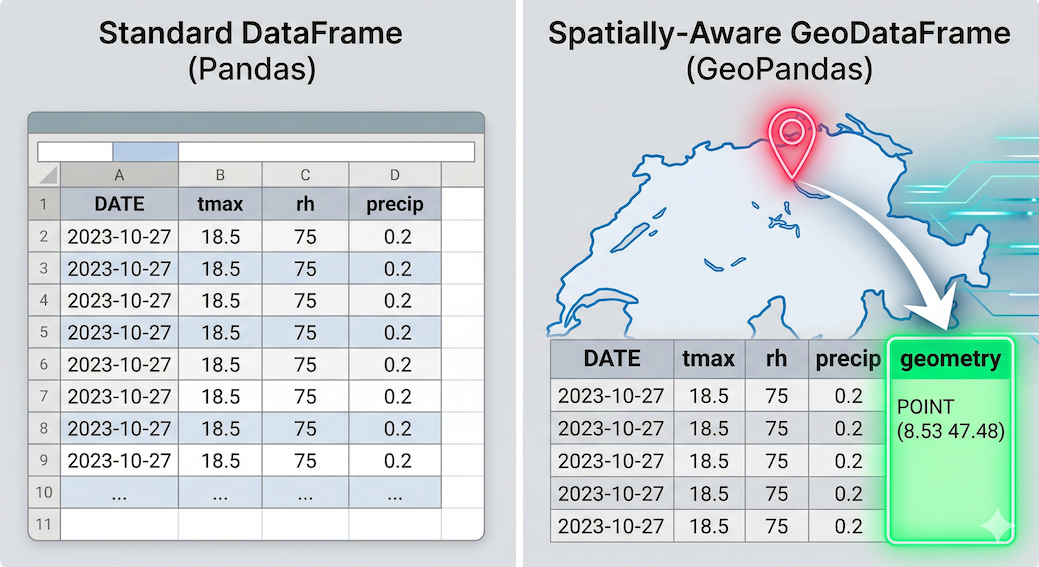
A side-by-side comparison showing a standard spreadsheet on the left, and a map of Switzerland connected to a table with a highlighted geometry column on the right. — *The transition from tabular data (Pandas) to spatially-aware data (GeoPandas). The geometry column acts as the bridge between raw numbers and physical geography.*

A GeoDataFrame solves this exact problem by adding a special, active geometry column.

Unlike standard columns that hold basic text or numbers, the geometry column holds mathematical shapes. When a DataFrame becomes a GeoDataFrame, it is no longer just a flat grid of numbers. It suddenly gains the ability to:

calculate physical areas and perimeters
measure exact distances to other geographic objects
plot itself directly onto a map

2. Under the Hood: Shapely Objects¶

GeoPandas does not actually do the spatial math itself. Creating and representing vector-based geometric objects is most commonly done using the Shapely library.

Under the hood, Shapely uses a highly optimized C++ library called GEOS to construct these geometries. This is the exact same engine that powers major professional GIS software like QGIS and PostGIS.

Shapely represents physical space using standardized geometric objects that adhere to Open Geospatial Consortium specifications. To understand vector data, you only need to understand three fundamental building blocks:

Point: Created by passing X and Y coordinates into the class constructor. Used for specific singular locations like a weather station or a city center.
LineString: Created using at least two points that are connected to each other. Used for linear features like rivers, roads, or GPS flight paths.
Polygon: Created using at least three coordinate tuples to form a closed surface. A Polygon can also contain optional interior rings to represent negative space or “holes” inside the shape. Used for areas like lakes or country borders.

Well-Known Text (WKT) and Visual Geometries¶

When computers communicate about these shapes, they often use a standardized string format called Well-Known Text (WKT). Below is a visual guide to how these 2D geometry primitives translate into WKT coordinates.

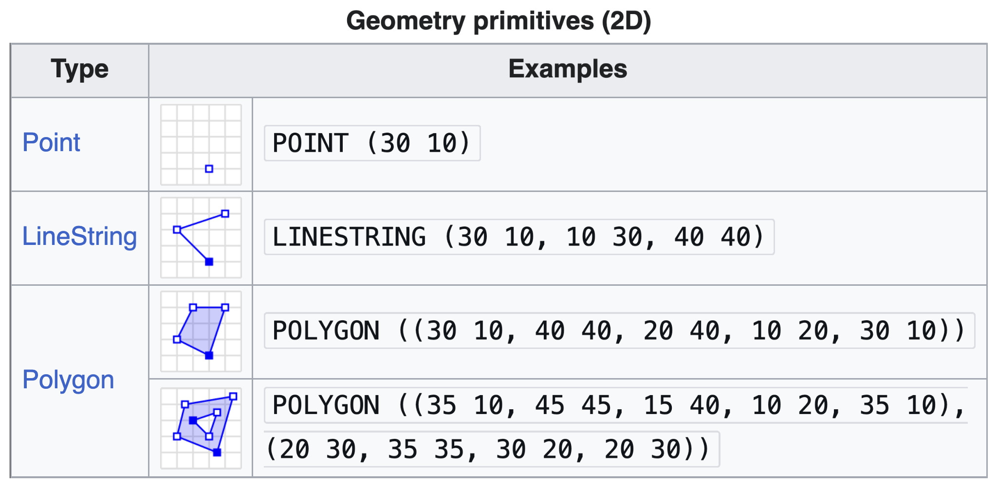
Diagrams showing a Point, LineString, a solid Polygon, and a Polygon with a hole on a Cartesian coordinate grid. — *Visual representation of the fundamental 2D geometry primitives. Source: Wikipedia*

Creating Geometries in Python¶

Because Shapely objects are mathematically aware, they come equipped with built-in attributes and methods. You can effortlessly extract their WKT representation, calculate a line’s length, or find the mathematical center (centroid) of a shape.

Let us look at how these geometries are constructed in pure Python:

from shapely.geometry import Point, LineString, Polygon

# 1. Point: A single coordinate pair (Longitude, Latitude)
point = Point(2.2, 4.2)

# 2. LineString: A connected sequence of points
line = LineString([(2.2, 4.2), (7.2, -25.1), (9.26, -2.456)])

# 3. Polygon: A closed sequence of points forming an area
poly = Polygon([(0, 0), (0, 4), (4, 4), (4, 0)])

# Every object can print its WKT representation
print(f"Point geometry: {point.wkt}")

# Objects know their own mathematical properties
print(f"Line length: {line.length:.2f} degrees")
print(f"Polygon area: {poly.area} square degrees")

Complex Entities (Multi-Geometries)¶

Sometimes, a single geographic entity is made up of multiple separate shapes. For example, a single country might be composed of several disconnected islands, or a single highway might break into separate segments.

Shapely handles this seamlessly using Multi counterparts: MultiPoint, MultiLineString, and MultiPolygon. You simply pass a list of individual points, lines, or polygons into these constructors to group them into a single coherent object.

Just like the fundamental primitives, these complex entities have standardized Well-Known Text (WKT) representations. Notice how the parentheses group the individual parts together!

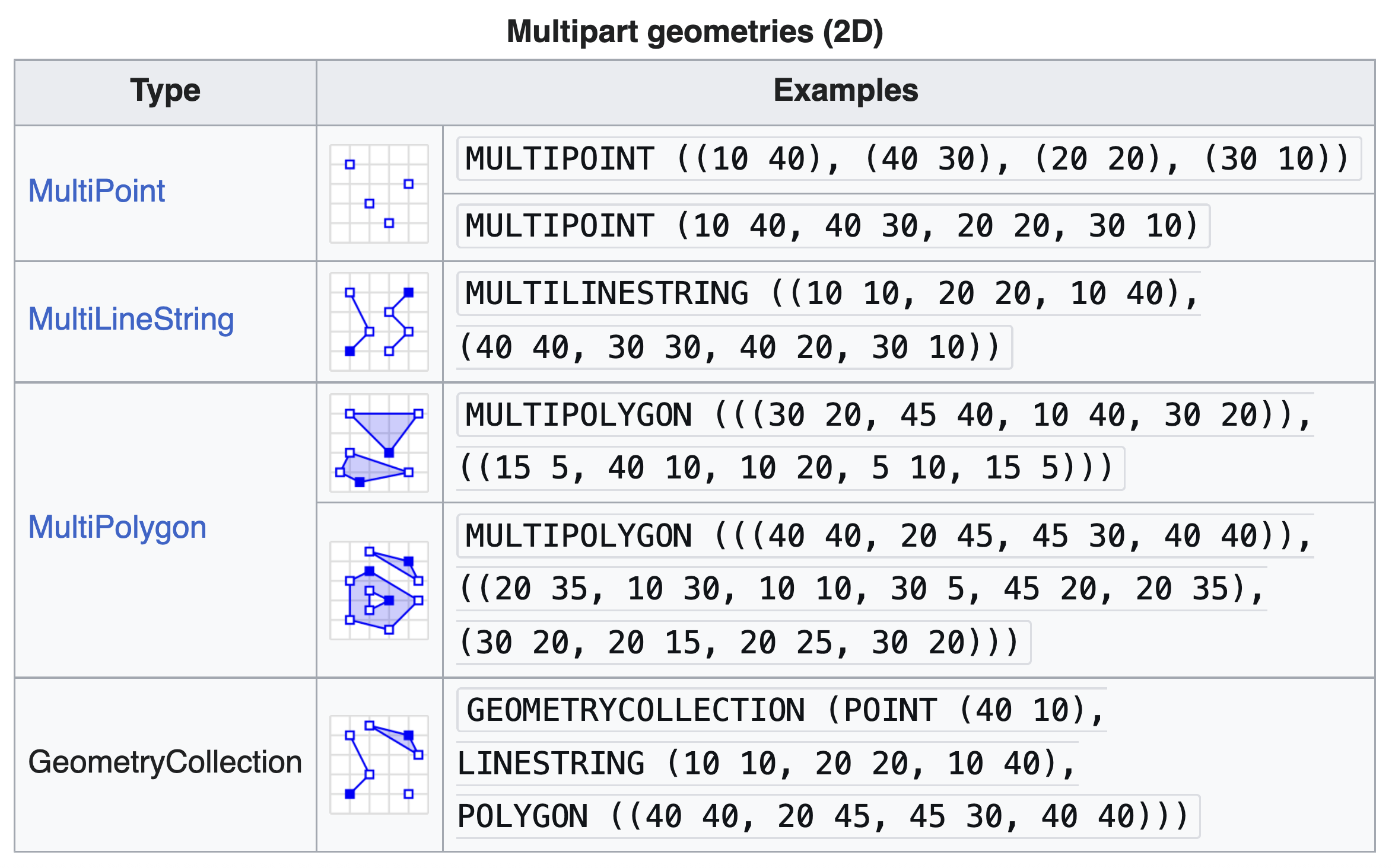
Diagrams showing MultiPoint, MultiLineString, and two MultiPolygons (one solid, one containing a hole) on a Cartesian coordinate grid. — *Visual representation of multi-part geometries. A single MultiPolygon object can represent multiple disconnected areas, and even contain holes. Source: Wikipedia*

Creating these in Python is just as straightforward as creating the primitives. You just wrap the individual geometries in a list:

from shapely.geometry import MultiPoint, MultiPolygon

# Grouping multiple Point objects into a single MultiPoint entity
multi_point = MultiPoint([Point(2, 2), Point(3, 3)])

# Grouping multiple Polygons into a single MultiPolygon entity
multi_poly = MultiPolygon(
    [
        Polygon([(0, 0), (0, 4), (4, 4), (4, 0)]),
        Polygon([(6, 6), (6, 12), (12, 12), (12, 6)]),
    ]
)

print(f"MultiPoint geometry: {multi_point.wkt}")
print(f"Total area of all polygons combined: {multi_poly.area} square degrees")

3. From Pandas to GeoPandas¶

Most spatial data you encounter in the wild will not start as a ready-to-use spatial file. Often, you will download a standard CSV file where the spatial information is just sitting in two basic text columns (typically labeled “Longitude/Latitude” or “X/Y”).

To demonstrate how to upgrade a standard table into a spatially aware object, we will use a dataset containing the Swiss pollen monitoring station network (meteoswiss_pollen_network.csv).

First, we load the CSV using standard Pandas:

import geopandas as gpd
import pandas as pd

# 1. Load the CSV as a standard Pandas DataFrame
pollen_df = pd.read_csv("meteoswiss_pollen_network.csv")

# Look at the data types
print("Original type:", type(pollen_df))
display(pollen_df.head(3))

Output:

Original type: <class 'pandas.core.frame.DataFrame'>

Standard Pandas DataFrame (pollen_df)

index	fid	id	station_name	altitude	X	Y
0	1	PLO	Locarno / Monti	376	2704158	1114348
1	2	PBS	Basel	256	2610935	1267909
2	3	PBE	Bern	546	2598936	1199918

Notice that the spatial data is currently trapped in the X and Y columns as basic numeric coordinates.

The Anatomy of the Transformation¶

Essentially, GeoPandas provides a high-level interface that extends the familiar Pandas data analysis framework to allow for geospatial operations.

A GeoDataFrame is basically like a standard pandas DataFrame, but it contains at least one dedicated column for storing geometries. This dedicated column is actually a GeoSeries data structure, which holds the geometries as Shapely objects (points, lines, polygons).

To transform our pollen data into a GeoDataFrame, we must tell GeoPandas to take the coordinate columns, fuse them into Shapely Point objects, and store them in a new GeoSeries column named geometry. We do this using the gpd.points_from_xy() function:

# 2. Convert the standard DataFrame into a GeoDataFrame
pollen_gdf = gpd.GeoDataFrame(
    pollen_df, geometry=gpd.points_from_xy(pollen_df["X"], pollen_df["Y"])
)

# Verify the transformation!
print("New type:", type(pollen_gdf))
display(pollen_gdf.head(3))

Output:

New type: <class 'geopandas.geodataframe.GeoDataFrame'>

Spatially-aware GeoDataFrame (pollen_gdf)

index	fid	id	station_name	altitude	X	Y	geometry
0	1	PLO	Locarno / Monti	376	2704158	1114348	POINT (2704158 1114348)
1	2	PBS	Basel	256	2610935	1267909	POINT (2610935 1267909)
2	3	PBE	Bern	546	2598936	1199918	POINT (2598936 1199918)

Congratulations! You have just created your first GeoDataFrame. Notice the brand new geometry column on the far right. It contains actual Shapely Point objects, meaning this data is now fully equipped for spatial analysis.

Concept Check: The Coordinate Order¶

When building Shapely points using gpd.points_from_xy(), you must provide the horizontal (X) coordinates first, and the vertical (Y) coordinates second.

If you are working with geographic data, which column represents X, and which represents Y?

Check your understanding

Longitude (or Easting) is X, and Latitude (or Northing) is Y.

This is a very common trap! People are used to saying “Latitude and Longitude” in everyday conversation. However, on a Cartesian grid, the horizontal axis (X) represents Longitude (moving East/West), and the vertical axis (Y) represents Latitude (moving North/South). Always pass the horizontal/Easting/Longitude column first!

4. The Active Geometry¶

A GeoDataFrame is essentially a standard Pandas DataFrame equipped with an active geometry column.

Because it retains its tabular core, a single GeoDataFrame can actually store multiple spatial features side-by-side. Imagine a dataset analyzing commuter trains: you could have one column of Point objects for the start_station, another column of Point objects for the end_station, and a LineString column representing the actual route_path.

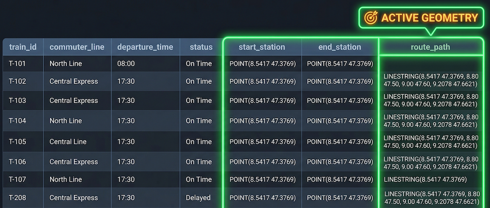
A data table containing three spatial columns: start_station, end_station, and route_path. Only the route_path column is highlighted with a bright bounding box and labeled as 'Active'. — *A single GeoDataFrame can store multiple spatial columns, but GeoPandas will only use the designated ‘Active Geometry’ for plotting and spatial operations.*

However, a GeoDataFrame can only have one active geometry at a time. This active column acts as the default spatial context. If you ask GeoPandas to plot the data, calculate an area, or measure a distance, it will automatically execute that command using the active geometry. By default, when you construct a GeoDataFrame, this active column is simply named geometry.

You can always check which column is currently powering the spatial engine using the .geometry.name attribute:

# Check which column is currently powering the spatial math
print("The active geometry column is:", pollen_gdf.geometry.name)

Output:

The active geometry column is: geometry

Switching the Spatial Context¶

If you have multiple geometry columns and you want to perform calculations on a different one, you do not need to create a brand new GeoDataFrame. You can dynamically switch the spatial context using the .set_geometry() method.

5. Exercise: Make it Spatial¶

It is time to put your new spatial mindset to the test. You have been provided with a standard CSV file containing the coordinates of nuclear power plants in Switzerland (NuclearPowerPlant.csv).

Your task is to ingest this purely tabular data, explore its structure, and upgrade it into a spatially aware GeoDataFrame.

Tasks:

Load: Read the CSV file using standard Pandas into a variable called power_plants_df.
Explore: Print the .columns of your new DataFrame to find out exactly what the coordinate columns are named (they might be X/Y, E/N, or Longitude/Latitude).
Upgrade: Convert the table into a GeoDataFrame called power_plants_gdf. Use gpd.points_from_xy() and pass the correct horizontal (X) and vertical (Y) columns you discovered in step 2.
Verify: Print the data type of power_plants_gdf to verify it is no longer a standard DataFrame.
Inspect: Display the first 3 rows to confirm the new geometry column exists. Finally, to tie it all together, print the name of the active geometry column!

# Write your code here

Sample solution

import pandas as pd
import geopandas as gpd

# 1. Load the raw tabular data
power_plants_df = pd.read_csv("NuclearPowerPlant.csv")

# 2. Explore the columns to find the coordinate names
print("Columns in CSV:", power_plants_df.columns.values)

# 3. Upgrade to a GeoDataFrame 
# (Assuming the print statement revealed columns named 'X' and 'Y')
power_plants_gdf = gpd.GeoDataFrame(
    power_plants_df,
    geometry=gpd.points_from_xy(power_plants_df["X"], power_plants_df["Y"])
)

# 4 & 5. Verify the spatial transformation and inspect
print("\nObject type:", type(power_plants_gdf))
print("Active geometry column:", power_plants_gdf.geometry.name)
display(power_plants_gdf.head(3))

(Note: Depending on the exact headers in the CSV, your column names for X and Y might be slightly different, such as ‘E’ and ‘N’ for Swiss coordinates. Always check your columns first!)

6. Summary: The Anatomy of a GeoDataFrame¶

In this section, you successfully shifted your mental model from flat spreadsheets to dynamic spatial objects.

Key takeaways¶

The Integration: GeoPandas is simply the powerful data manipulation of Pandas fused with the geometric mathematics of Shapely. Everything you learned in the previous lesson (filtering, slicing, vectorization) still works perfectly on a GeoDataFrame!
Shapely Objects: Vector data is constructed from mathematical shapes: Points (locations), LineStrings (paths), Polygons (areas), and their complex Multi-part combinations.
The Conversion: You can easily upgrade a standard CSV with coordinates into a spatial dataset using gpd.GeoDataFrame() combined with gpd.points_from_xy(). Remember the coordinate order trap: horizontal (X/Longitude/Easting) always comes before vertical (Y/Latitude/Northing)!
Active Geometry: A table can store multiple geographic features side-by-side, but it relies on a single “active” geometry column to execute spatial commands like measuring distances or mapping.

What comes next?¶

Now that you understand the anatomy of a GeoDataFrame, how do we actually load professional GIS files? We rarely build spatial datasets from raw CSVs in the real world.

In the next section, Reading, Writing, and Peeking at Spatial Data, we will learn how effortlessly Python handles complex industry-standard formats (like Shapefiles, GeoJSON, and GeoPackages), how to instantly verify your data visually using the .plot() method, and how to export your modified maps back to your hard drive!