
Before we begin, make sure you have downloaded the necessary datasets for this section. We will be using one familiar and two new Kloten datasets, plus a new dataset from Säntis.
In data science workflows, there are many ways to represent time (such as Python’s built-in datetime module or NumPy’s datetime64). However, we will standardize on Pandas datetime objects (pd.Timestamp). Pandas handles time seamlessly, works perfectly with DataFrames, and includes powerful tools for manipulating time series data.
(Note: You may encounter other datetime types in legacy Python code, but Pandas can automatically convert and handle them in almost all workflows!)
To explore these temporal superpowers, let us start by loading our familiar daily weather dataset from Kloten.
import pandas as pd

# Load the daily Kloten dataset
fp = "kloten_summer_2022_extended.txt"
data = pd.read_csv(fp, sep=r"\s+", skiprows=[1], na_values=["-9999"])

# Let us ensure our DATE column is treated as text (a string) for now
data["DATE"] = data["DATE"].astype(str)

display(data[["DATE", "tmean"]].head(3))
1. The Problem with Strings as Dates
When you look at the DATE column, you see a date: June 1st, 2022 ("20220601").
However, your computer does not see a date. Because this column is formatted as a string (text), the computer sees a meaningless collection of characters. To Python, "20220601" is functionally no different than the word "Banana".
This creates a massive problem for data analysis. What if we wanted to calculate exactly how many days our summer dataset covers by subtracting the first date from the last date? Let’s see what happens if we try to do math with strings:
# Grab the very last date in the dataset
last_date = data["DATE"].iloc[-1]

# Grab the very first date
first_date = data["DATE"].iloc[0]

# Attempt to calculate the duration
duration = last_date - first_dateYou cannot subtract "Banana" from "Apple", and therefore, Python cannot subtract "20220601" from "20220831".
Furthermore, keeping dates as strings creates dangerous traps for chronological sorting. While a string like YYYY-MM-DD happens to sort correctly alphabetically, a date formatted like DD-MM-YYYY will sort completely out of order (e.g., "01-12-2022" will be placed before "02-01-2022", tricking your computer into thinking December comes before January!).
To perform real temporal analysis—like calculating durations, sorting chronologically, or plotting accurate time series graphs—we must translate these useless strings into a format that mathematically understands the rules of time.
2. Converting to Datetime
To fix our math error and perform real time series analysis, we need to translate our text strings into a format that the computer recognizes as time.
Pandas provides a dedicated function for this called pd.to_datetime(). It takes an entire column of text strings, analyzes the characters, and intelligently parses them into specialized time-aware objects called datetime64.
Let us overwrite our broken string column with these new datetime objects, and try our math calculation one more time!
# 1. Convert the string column to official Pandas datetime objects
data["DATE"] = pd.to_datetime(data["DATE"])

# 2. Let us check the new data type
print("New data type:", data["DATE"].dtypes)

# 3. Try the exact same math that failed in the previous section!
last_date = data["DATE"].iloc[-1]
first_date = data["DATE"].iloc[0]

duration = last_date - first_date
print(f"The dataset covers a duration of: {duration}")It worked! Because the data is now stored as datetime64, Pandas mathematically understands the rules of the calendar. When you subtract two dates, it successfully returns a Timedelta object (representing an exact duration of time) showing us our summer dataset spans exactly 91 days.
Custom Date Formats
In the example above, Pandas was smart enough to automatically figure out that "20220601" meant Year-Month-Day. However, real-world data is often messy. You might encounter European dates ("31.12.2022"), US dates ("12/31/2022"), or highly detailed timestamps ("2020-12-22T15:00:00").
If Pandas cannot automatically guess the format—or worse, if it guesses incorrectly by mixing up days and months—you must explicitly tell it how to read the string by providing a format argument.
The Formatting Rule: You build the format string by replacing the date values with special directives (codes starting with %), while keeping all original separators (spaces, dashes, colons, slashes) exactly the same.
For example, how would we parse the human-written date "22 December 2020"?
22is the zero-padded day of the month%dDecemberis the full month name%B2020is the 4-digit year%YThey are separated by spaces, so our final format is
"%d %B %Y".
Let us see this in action:
# Create a tiny DataFrame with a very strange, human-written date format
messy_data = pd.DataFrame({"messy_date": ["22 December 2020", "01 January 2021"]})

# Explicitly tell Pandas how to parse this specific string structure
messy_data["clean_date"] = pd.to_datetime(messy_data["messy_date"], format="%d %B %Y")

display(messy_data)
Output of custom datetime parsing
| messy_date | clean_date | |
|---|---|---|
| 0 | 22 December 2020 | 2020-12-22 00:00:00 |
| 1 | 01 January 2021 | 2021-01-01 00:00:00 |
To parse any temporal text you encounter in the wild, simply match the characters to the standard directives below.
You can find a more complete table in the official pandas.Period.strftime documentation.
Most commonly used datetime directives
| Directive | Description | Examples |
|---|---|---|
%Y | Year including century (4 digits) | 2020, 1999 |
%y | Year without century (2 digits) | 20, 99 |
%m | Month as a zero-padded number | 01, ..., 12 |
%B | Month as full name | January, December |
%b | Month as abbreviated name | Jan, Dec |
%d | Day of the month | 01, ..., 31 |
%H | Hour (24-hour clock) | 00, ..., 23 |
%M | Minute | 00, ..., 59 |
%S | Second | 00, ..., 59 |
Concept Check: Decoding human-entered data
You receive a messy dataset where a colleague manually typed the dates and times into a spreadsheet. The timestamps look like this: "July 14, 2024 (14:30)".
How would you write the format= string inside pd.to_datetime() to successfully parse this?
Check your understanding
format="%B %d, %Y (%H:%M)"
Why? You must use the specific directive for a full month name (%B), and explicitly include every single space, comma, and parenthesis exactly where they appear in the original text!
The Pro-Trick: parse_dates
Using pd.to_datetime() after loading your data is perfectly fine. However, professional data scientists usually prefer to fix their dates at the exact moment they read the file.
The pd.read_csv() function has a built-in parameter called parse_dates. If you hand it a list of column names, Pandas will automatically convert those columns into datetime64 objects as the file is being loaded, saving you an entire step of data cleaning!
Let us reload our dataset one last time, using the pro-trick to get it perfectly clean from the start.
# The cleanest way to load temporal data
fp = "kloten_summer_2022_extended.txt"

data = pd.read_csv(
    fp,
    sep=r"\s+",
    skiprows=[1],
    na_values=["-9999"],
    parse_dates=["DATE"],  # <-- The magic parameter!
)

# Verify it worked automatically
display(data[["DATE", "tmean"]].head(3))
print("Column type:", data["DATE"].dtypes)
Output of parse_dates
| DATE | tmean | |
|---|---|---|
| 0 | 2022-06-01 | 14.8 |
| 1 | 2022-06-02 | 17.0 |
| 2 | 2022-06-03 | NaN |
Column type: datetime64[ns]Notice how the DATE column in the table now has dashes (2022-06-01) instead of being crammed together (20220601)? That is the visual confirmation that Pandas has successfully parsed your text into a fully functioning datetime object.
Concept Check: Decoding the format
You receive a messy dataset from a faulty weather sensor where the timestamps look like this: "2024_07_14-08:30".
How would you write the format= string inside pd.to_datetime() to successfully parse this?
Check your understanding
format="%Y_%m_%d-%H:%M"
Why? You must keep the exact separators (the underscores and the dash) in the exact same positions as the original text, while replacing the numbers with their respective % directives.
3. Extracting Time Components
In an earlier lesson, we extracted the month from a date by slicing the text string (e.g., .str.slice(4, 6)). While that works for perfectly formatted text, it is rigid and prone to errors.
Because we converted our column to official datetime64 objects in the previous step, we no longer need to slice strings. Instead, we can use Pandas’ special datetime accessor: .dt.
The .dt accessor acts like a master key, allowing you to instantly pull out the year, month, day, or even the day of the week, mathematically and accurately.
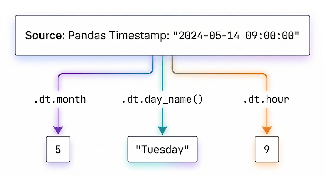
Figure 1:The .dt accessor extracts specific temporal components from a full timestamp.
To see the true power of this, let us switch to a higher-resolution dataset. We will load hourly weather data for the spring of 2024 (kloten_spring_2024_hourly.csv), remembering to use our parse_dates trick right from the start!
# 1. Load the hourly dataset and instantly parse the timestamp
hourly_data = pd.read_csv("kloten_spring_2024_hourly.csv", parse_dates=["timestamp"])

# 2. Extract components into brand new columns using the .dt accessor
hourly_data["month"] = hourly_data["timestamp"].dt.month
hourly_data["day_of_week"] = hourly_data["timestamp"].dt.day_name()
hourly_data["hour"] = hourly_data["timestamp"].dt.hour

# 3. View a random sample of 3 rows to see our new columns
display(hourly_data[["timestamp", "month", "day_of_week", "hour"]].sample(3))
Output of .dt extraction
| timestamp | month | day_of_week | hour | |
|---|---|---|---|---|
| 1041 | 2024-05-14 09:00:00 | 5 | Tuesday | 9 |
| 771 | 2024-05-03 03:00:00 | 5 | Friday | 3 |
| 1376 | 2024-05-28 08:00:00 | 5 | Tuesday | 8 |
The Payoff: Plotting the Diurnal Cycle
Extracting the hour might seem like a small trick, but it unlocks incredible analytical power when combined with the .groupby() method we learned in the previous lesson.
If we group our entire spring dataset by the newly extracted hour column, we can calculate the average temperature for every single hour of the day across the entire season. This reveals the diurnal temperature cycle (the natural fluctuation of temperature between day and night).
Let us calculate it and plot the results!
# 1. Group by the hour and calculate the mean temperature
diurnal_cycle = hourly_data.groupby("hour")["temperature"].mean()

# 2. Plot the results
ax = diurnal_cycle.plot(
    figsize=(8, 4),
    title="Average Diurnal Temperature Cycle (Kloten, Spring 2024)",
    xlabel="Hour of the Day (0-23)",
    ylabel="Average Temperature (°C)",
    linewidth=2,
    marker="o",  # Add dots for each specific hour
    color="darkorange",
)
# Add a grid and set the bottom axis to show every 2 hours
ax.grid(True, linestyle="--", alpha=0.7)
ax.set_xticks(range(0, 24, 2));
(When you run this code, you should see a beautiful, smooth bell curve where temperatures are coldest around sunrise (04:00 - 05:00) and peak in the afternoon (14:00 - 15:00)!)
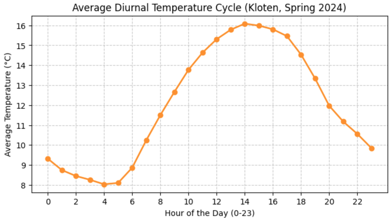
Figure 2:The average diurnal temperature cycle calculated by grouping hourly data. Temperatures drop to their lowest right before sunrise and peak in the afternoon.
4. The DatetimeIndex and Time Slicing
In previous lessons, we used .loc[] to select rows by checking conditions (e.g., data.loc[data["month"] == 5]). While this works, it requires writing out full logical statements.
When working with time series, there is a much more elegant way. The ultimate Pandas time-series trick is to set your datetime column as the DataFrame’s index.
Let us take our hourly_data from the previous section and move the timestamp column into the index position:
# Set the timestamp column as the index
hourly_data = hourly_data.set_index("timestamp")

# Notice how 'timestamp' drops down a level to become the index!
display(hourly_data.head(3))
Output of set_index
| temperature | precipitation | sunshine_duration | month | day_of_week | hour | |
|---|---|---|---|---|---|---|
| timestamp | ||||||
| 2024-04-01 00:00:00 | 10.6 | 0.0 | 0 | 4 | Monday | 0 |
| 2024-04-01 01:00:00 | 10.2 | 0.0 | 0 | 4 | Monday | 1 |
| 2024-04-01 02:00:00 | 9.0 | 0.0 | 0 | 4 | Monday | 2 |
Partial String Indexing
Now that our DataFrame is equipped with a DatetimeIndex, it unlocks a superpower called partial string indexing.
You no longer need to write complex logical rules to filter your data. You can simply pass a string representing the year and month to .loc[], and Pandas is smart enough to instantly grab every single row that belongs to that month!
# Effortlessly select all 744 hourly observations from exactly May 2024
may_data = hourly_data.loc["2024-05"]

print(f"May 2024 contains {len(may_data)} hourly observations.")Time Slicing
This string indexing also works flawlessly for ranges (slicing).
Imagine you wanted to analyze the weather during the first week of April. Instead of trying to calculate exactly which index row numbers correspond to those days, you just pass the start and end dates separated by a colon (:).
# Slice a specific week of data (April 1st through April 7th)
# Note: With .loc slicing, the end date is INCLUDED!
first_week_april = hourly_data.loc["2024-04-01":"2024-04-07"]

# Calculate the total precipitation for that specific week
total_rain = first_week_april["precipitation"].sum()

print(f"Total rows extracted: {len(first_week_april)}")
print(f"Total rain for the first week of April: {total_rain} mm")By putting time in the index, your DataFrame is now fundamentally “time-aware,” allowing you to slice, filter, and navigate your dataset using natural dates instead of arbitrary row numbers.
Concept Check: Inclusive or Exclusive?
In standard Python lists, slicing is “exclusive” at the end (e.g., my_list[0:5] grabs indices 0, 1, 2, 3, and 4, but stops before 5).
If your DataFrame has a DatetimeIndex and you use the command .loc["2024-04-01":"2024-04-07"], does the resulting dataset include the observations from April 7th?
Check your understanding
Yes, April 7th is completely included! When slicing with .loc[] and a DatetimeIndex, Pandas uniquely includes the final boundary. It will grab everything up until the very last millisecond of April 7th. It is important to remember this difference so you do not accidentally analyze an extra day of data!
5. Time Travel: Shifting and Resampling
Working with time series often means moving between different temporal resolutions or comparing a moment in time to the past. Pandas provides two incredibly powerful methods for these “time travel” operations: .resample() and .shift().
Resampling (Changing Frequency)
Environmental sensors often record data at very high frequencies (like our hourly Kloten spring dataset). However, you usually want to analyze broader daily or monthly trends.
To downsample your data (change it to a lower frequency), Pandas provides the .resample() method. It works exactly like the .groupby() method we learned earlier, but it is specifically designed to slice data along time boundaries!
Let us take our hourly_data (which already has the timestamp as its index) and aggregate it into daily summaries.
# 1. Resample hourly precipitation into Daily ('D') buckets and calculate the SUM
daily_rain = hourly_data["precipitation"].resample("D").sum()

# 2. Resample hourly temperatures into Daily ('D') buckets and calculate the MEAN
daily_temp = hourly_data["temperature"].resample("D").mean()

print("Total Daily Rainfall (mm):")
display(daily_rain.head(3))Notice that you must choose the correct mathematical function for your variable! Taking the sum of daily rainfall makes scientific sense, while taking the sum of hourly temperatures would be meaningless (which is why we use .mean() for temperature).
Shifting (Lagging Data)
Sometimes you do not want to aggregate data; you want to compare a row to the row immediately before it. A classic meteorological question is: “How much did the maximum temperature drop since yesterday?”
Pandas uses the .shift() method to push data down by a specified number of rows.
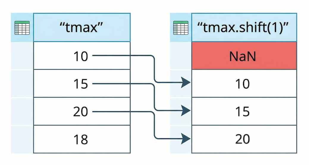
Figure 3:The .shift(1) operation lags data by pushing all values down one row. The empty space created at the top is automatically filled with a NaN (Not a Number) value.
To demonstrate this, let us load a massive new dataset: the historical daily records for Kloten spanning over 40 years (kloten_daily_19800101_20260101.csv).
# 1. Load the historical daily dataset, parse the dates, and set the index
fp_daily = "kloten_daily_19800101_20260101.csv"
historical_data = pd.read_csv(fp_daily, parse_dates=["DATE"])
historical_data = historical_data.set_index("DATE")

# 2. Create a "Yesterday" column by shifting the tmax data down by 1 row
historical_data["tmax_yesterday"] = historical_data["tmax"].shift(1)

# 3. Calculate the day-to-day temperature swing
historical_data["temp_swing"] = (
    historical_data["tmax"] - historical_data["tmax_yesterday"]
)

# View the first few rows to see the shift in action!
columns_to_show = ["tmax", "tmax_yesterday", "temp_swing"]
display(historical_data[columns_to_show].head(4))
Output of shifting data
| DATE | tmax | tmax_yesterday | temp_swing |
|---|---|---|---|
| 1980-01-01 | 0.1 | NaN | NaN |
| 1980-01-02 | 5.7 | 0.1 | 5.6 |
| 1980-01-03 | 9.7 | 5.7 | 4.0 |
| 1980-01-04 | 14.7 | 9.7 | 5.0 |
Notice the first row! Because we shifted the data forward by exactly one day, there is no “yesterday” available for the very first observation (January 1st, 1980), so Pandas correctly fills it with NaN.
By subtracting the shifted column from the original column, we instantly calculated the day-to-day temperature swings for over 40 years of data without writing a single for loop!
6. Smoothing with Rolling Statistics
If you plot daily environmental data over a long period, the result often looks like a solid wall of static. Weather is inherently “noisy”—temperatures swing wildly from day to night and from week to week, making it very difficult to spot larger climate patterns.
To reveal the underlying signal hidden in the noise, we can calculate a moving average (also known as a rolling average).
Pandas provides the .rolling() method for this exact purpose. It creates a sliding window that moves down your time series, averaging a set amount of past observations together. This smooths out short-term fluctuations and highlights longer-term trends.
Let us use our 40-year historical dataset to see this in action. Because our DataFrame has a DatetimeIndex, we do not have to guess row numbers; we can just pass a string representing the time window we want (e.g., "365D" for a one-year window)!
# 1. Calculate a 1-year rolling average (smooths out daily weather, shows yearly cycles)
historical_data["1_year_trend"] = historical_data["tmean"].rolling("365D").mean()

# 2. Calculate a 10-year rolling average (smooths out yearly cycles, shows climate change)
# Note: 10 years is roughly 3650 days
historical_data["10_year_trend"] = historical_data["tmean"].rolling("3650D").mean()

# 3. View the first few rows
display(historical_data[["tmean", "1_year_trend", "10_year_trend"]].head(5).round(2))
Output of rolling averages
| DATE | tmean | 1_year_trend | 10_year_trend |
|---|---|---|---|
| 1980-01-01 | -1.7 | -1.70 | -1.70 |
| 1980-01-02 | 3.4 | 0.85 | 0.85 |
| 1980-01-03 | 2.2 | 1.30 | 1.30 |
| 1980-01-04 | 10.4 | 3.58 | 3.58 |
| 1980-01-05 | 11.6 | 5.18 | 5.18 |
(Note: Because we used a time-based window like "365D", Pandas starts calculating the average immediately using whatever data it has so far. If we had used a strict row count like window=365, the first 364 rows would simply be NaN!)
Concept Check: Resample or Rolling?
Imagine you are analyzing highly detailed hourly weather data.
Scenario A: You want to calculate the total precipitation that fell on each individual day to find out which day of the month was the wettest. Scenario B: You want to smooth out the hourly temperature fluctuations to create a continuous trendline that still has an hourly resolution.
Which Pandas time-travel method (.resample() or .rolling()) should you use for each scenario?
Check your understanding
Scenario A requires .resample(). Resampling groups the data into discrete “buckets” and fundamentally changes the frequency of the dataset (e.g., collapsing 24 hourly rows into 1 single daily row).
Scenario B requires .rolling(). Rolling calculates a moving average over a sliding window, but it keeps the original number of rows. The frequency stays hourly, but the values are smoothed out based on their neighbors.
Visualizing the Climate Trend
Now for the payoff. Let us plot our raw, noisy daily temperatures in a light, transparent color, and overlay our newly calculated rolling averages to see the true trajectory of Kloten’s climate since 1980.
# 1. Plot the raw daily data (faint gray)
ax = historical_data["tmean"].plot(
    figsize=(12, 6),
    color="lightgray",
    alpha=0.5,  # Make it partially transparent
    label="Daily Mean (Raw Weather)",
)
# 2. Add the 1-year rolling average (blue)
historical_data["1_year_trend"].plot(
    ax=ax, color="dodgerblue", linewidth=1.5, label="1-Year Trend"
)
# 3. Add the 10-year rolling average (red)
historical_data["10_year_trend"].plot(
    ax=ax, color="crimson", linewidth=3, label="10-Year Climate Trend"
)
# 4. Add styling and labels
ax.set_title("40-Year Temperature Trends in Kloten (1980 - 2026)", fontsize=14)
ax.set_ylabel("Temperature (°C)", fontsize=12)
ax.set_xlabel("Date", fontsize=12)
ax.legend()
When you run this code, the visual story becomes undeniable. The gray static represents the chaotic daily weather. The blue line oscillates up and down, showing the reliable shift between warm summers and cold winters. But the thick red line cuts through all the noise, revealing a clear, upward trajectory in the baseline average temperature over the last 40 years.
By mastering time series data, you are no longer just cleaning spreadsheets—you are analyzing the Earth’s shifting climate.
Quantifying the Trend
Visualizing the red line going up is powerful, but as data scientists, we want to put a hard number on it. Exactly how much is the temperature rising per year?
To find out, we can calculate a linear trendline (the slope). The easiest way to do this is to take our daily data, resample it into annual averages, and then use a mathematical function from the NumPy library to calculate the slope of the line.
import numpy as np

# 1. Resample the data to Annual ('YE') averages ('YE' = Year-End)
# This removes all the seasonal noise and gives us one temperature per year
annual_temps = historical_data["tmean"].resample("YE").mean().dropna()

# 2. Create a simple array representing the passing years (0, 1, 2, 3...)
years_passed = np.arange(len(annual_temps))

# 3. Use NumPy to fit a straight line (a 1st-degree polynomial) to the data
# This returns the slope (m) and the intercept (b) of the line
slope, intercept = np.polyfit(years_passed, annual_temps, 1)

print(f"The long-term warming trend is {slope:.3f}°C per year.")
print(f"Total warming over the dataset: {(slope * len(years_passed)):.2f}°C")With just three lines of code, we moved beyond just looking at a chart and mathematically proved the climate in Kloten is warming by a measurable fraction of a degree every single year.
7. Exercise: Temporal Superpowers
It is time to put your new time series skills to the test.
For this final challenge, we will start with a personal investigation using the Kloten dataset, and then move to the extreme environment of Säntis, a weather station located at the peak of a 2,500-meter high mountain in the Swiss Alps!
Task 1: The Birthday Weather
In Section 6, we loaded the 40-year historical dataset for Kloten (historical_data) and set the DATE column as the index.
Because your DataFrame is now “time-aware”, you can instantly look up the exact weather on the day you were born!
Use .loc[] to slice your exact birthday from the historical_data DataFrame and find out if it was raining or sunny.
Can you also solve what day of the week were you born using the .day_name() method?
# Write your code here:
Task 2: Load and Prepare the Alpine Data
Now, let us analyze the Säntis mountain dataset (saentis_hourly_temp_precip_20200101_20260101.csv).
Load the CSV file.
Ensure the
timestampcolumn is parsed as datetime objects right from the start.Set the
timestampcolumn as the DataFrame’s index.Display the first 2 rows to check your work.
# Write your code here:
Task 3: Resample and Plot
The data is currently hourly. That is far too detailed to see the seasonal shifts.
Resample the hourly
temperaturedata into monthly averages ("MS"or"M").Plot the resulting monthly averages as a line chart.
# Write your code here:
Task 4: Find the Extremes
Using your newly resampled monthly_saentis data, can you find the exact month that had the absolute highest average temperature?
(Hint: The .idxmax() method will return the index label—in this case, the date—of the highest value!)
# Write your code here:
8. Summary: Time-Aware Data Science
Congratulations! You have graduated from treating dates as meaningless text to mastering time series analysis.
Time is a fundamental dimension in environmental data. By structuring your DataFrames to be “time-aware,” you can manipulate thousands of records with elegance.
Key Takeaways
Conversion is Key: Always use
pd.to_datetime()or theparse_datesparameter inread_csv()to transform text intodatetime64objects.Component Extraction: The
.dtaccessor acts as a master key, allowing you to instantly pull out the year, month, hour, or day of the week.The DatetimeIndex: Using
.set_index()on your time column unlocks partial string indexing (e.g.,data.loc["2022-07"]), saving you from writing messy logical filters.Time Travel Tools: * Use
.resample()to change the frequency of your data (e.g., grouping hourly sensor data into daily summaries).Use
.shift()to push data forward or backward to calculate day-to-day differences.Use
.rolling()to calculate moving averages and expose long-term climate trends hidden inside noisy weather data.